Category Archives: Control

UDP Server C++ Class with a listening thread

DO NOT USE THIS CODE ANY LONGER. TOO MUCH OUTDATED AND BUGGY

I am sharing a code for “UDP Server C++ Class with a listening thread”. In the class “UDPThread”, a thread is running to receive a UDP packet.

Just compile a demo program with this command. Then you will understand.

g++ demo_udp_server.cpp UDPThread.cpp -lpthread -o demo_udp_server

This is the result.

I hope this code helps your project.

-Mok-

Minimal c++ class for Maxon EPOS2

1 Reply

Minimal c++ class for Maxon EPOS2

I am sharing the minimal C++ class for Maxon EPOS2. It includes a basic “initialization”, “Move”, “Read position”, “Close device” functions. The program consists of a class called “cmaxonmotor”. You can download the class and demo program here

You can see a simple demo program here.

#include <stdio.h>
#include <iostream>
#include "cmaxonmotor.h"

using namespace std;

int main(int argc, char *argv[])
{
    CMaxonMotor motor("USB0",1);
    motor.initializeDevice(); // initialize EPOS2

    long TargetPosition = -200000;
    int CurrentPosition = 0;

    motor.Move(TargetPosition); // move to the target position

    cout << "Press <Enter> to stop and quit..." << endl;
    getchar();
    motor.GetCurrentPosition(CurrentPosition); // get the current position
    cout << "Current Position: " << CurrentPosition << endl;

    motor.closeDevice(); // close EPOS2

    return 0;
}

You can control one motor just via USB, and also able to control multiple motors via USB-CAN gateway. For this version, see this article.

I hope this helps your project.

-Mok-

Sliding Mode Control (SMC), Robust control algorithm for nonlinear system

5 Replies

In this article, I am going to write about the Sliding Mode Control (SMC) algorithm.

Sliding Mode Control algorithm is a robust controller for nonlinear systems.

Robust control means that even though the system model has a certain error, if the controller can control the system, we say that the controller is robust.

SMC has two fundamental ideas.

1. To attract the system states to the surface.

2. To make the state slide on the surface toward the origin.

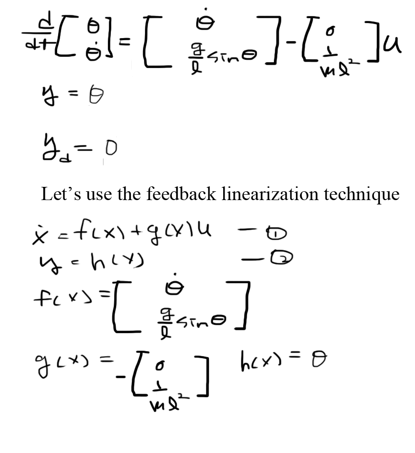
To explain the above two ideas more easily, let’s assume a typical control problem.

$\dot x = f_1 (x,\dot x)$ — (1)

$\ddot x = f_2 (x, \dot x) + u$

$y=Cx$ — (2) if it is nonlinear, you need to know Lie Derivatives.

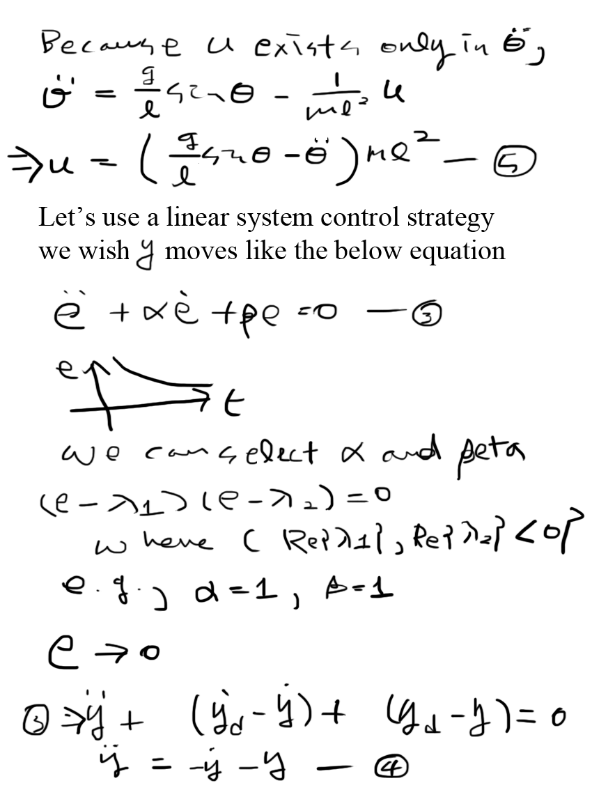
To achieve the first idea, we need to define a surface like the below. (Let’s assume that $y$ is a scalar and differentiable.)

$s(x)=a_0 e + a_1 \dot{e}$ where $e=y-y_d$ — (3)

Here we need to select a_0 and a_1 to make y->0 as t-> inf,s=0. You will see the reason after more several lines.

Let’s take the derivative of s(x) w.r.t. x. Then we can get the below equation.

$\dot{s}(x)=a_0 \dot e + a_1 \ddot e$ — (4)

In addition, if we add the additional term – $\eta \text{sign}(s)$ we can obtain the below equation,

$\dot{s}(x)=a_0 \dot e + a_1 \ddot e=-\eta \text{sign}(s)$ — (5)

Through a simple Lyapunov theorem, we can easily prove s-> 0 at t->inf .

if s=0, e-> 0 and \dot(e)-> 0, because we selected a_0 and a_1 to be like this.

Let’s look at (5),

$a_0 \frac{d}{dt}(y-y_d)+a_1 \frac{d^2}{dt^2}(y-y_d)=-\eta \text{sign}(s)$

=> $C(a_0 \dot x +a_1 \ddot x)=-\eta \text{sign}(s)$

=> $C(a_0 f_1 +a_1 (f_2+u)))=-\eta \text{sign}(s)$

=> $u=((-\eta \text{sign} (s))/C - a_0 f_1)/a_1 -f_2$

With this control input, we can control a nonlinear system with SMC.

it is difficult to explain quickly within short explanations…., if you need more explanation or questions, please leave me a reply.

Phase plane analysis and Matlab code toolbox

How to draw?

Given,

$\dot{x}_1=f_1(x_1,x_2)$

$\dot{x}_2=f_2(x_1,x_2)$

we can find the below equation

$\frac{dx_2}{dx_1}=\frac{f_2(x_1,x_2)}{f_1(x_1,x_2)}$

From $\frac{dx_2}{dx_1}$ , we can find the direction of the phase change at the point of $(x_1, x_2)$ .

Advantage:

It is an exact method. We can see the change of system’s state including transient response.
Simple graphical method. It is very intuitive and easy to understand its characteristics.

Limit:

Limited to the 2nd order system. It is expandable, but hard to visualize.

Reference

1. Lecture of Prof. Fernadez in Mech. Eng, The Univ. of Texas at Austin.

Extended Luenberger Observer for nonlinear system control

7 Replies

——————————————————————————————————————————–

Herman (who commented for this posting) told me that there are two different versions of ELO. One is just to linearize a nonlinear function (this posting will handle it), and the other is using Lie-algebraic approach (refer to M. Zeitz 1987 “The extended Luenberger Observer”).

Thank you Herman.

——————————————————————————————————————————–

This article is to explain the use of Luenberger observer for nonlinear system control. In other words, it is Extended Luenberger Observer, (ELO, just like Kalman Filter (KF), and Extended KF).

The basic idea is to linearize nonlinear system around the interesting point. The below is the description of ELO and how to select gain values for Extended Luenberger Observer. The below description assumes that you already know about Luenberger Observer for linear system. If you don’t know visit here.

I wish this can help your understanding about Luenberger observer, if you have any question, please leave me a comment below.

—————————————————————————————————————————–

I am Youngmok Yun, and writing about robotics theories and my research.

My main site is http://youngmok.com, and Korean ver. is http://yunyoungmok.tistory.com.

—————————

Luenberger observer for linear system control

1 Reply

This article explains the design of Luenberger observer for linear system control. If you are interested in the design of nonlinear system observer, read the next article. Observer in control systems is very important because we cannot directly “observe” the system state. One very popular observer is Kalman Filter and another is this Luenberger observer. Kalman Filter is built based on Bayesian rule (probabilistic) so that it is robust for measurement error, but slow. In contrast, Luenberger observer is based on deterministic sense so that fast. Of course, robustness is very important but robust measurement algorithm makes the algorithm slow, and actually Luenberger observer can observe most of systems successfully. The below is the proof and the selection of gain values for Luenberger observer, If you are interested in nonlinear version of Luenberger observer, read here.

I wish this can help your understanding about Luenberger observer, if you have any question, please leave me a comment below.

—————————————————————————————————————————–

I am Youngmok Yun, and writing about robotics theories and my research.

My main site is http://youngmok.com, and Korean ver. is http://yunyoungmok.tistory.com.

—————————————————————————————————————————–

Feedback linearization control (FBL) for nonlinear system control proof, practical implementation, and easy example part 2

Feedback linearization control (FBL) for nonlinear system control proof, practical implementation, and easy example part1

1 Reply

This article explains about Feedback linearization control (FBL) method for control of a nonlinear system. This is one of the easiest strategy to control nonlinear systems, but pretty powerful. The basic idea is that we can cancel control input by manipulating control input. The below is its proof.

This is the most basic concept to explain easily. If the nonlinear system is not fully controllable, we should use another strategy which finds reduced order manifold (ROM). About the more advanced technique and examples will be explained in the next articles.

—————————————————————————————————————————–

I am Youngmok Yun, and writing about robotics theories and my research.

My main site is http://youngmok.com, and Korean ver. is http://yunyoungmok.tistory.com.

—————————————————————————————————————————–

Youngmok Yun: Roboticist in Austin

Category Archives: Control

UDP Server C++ Class with a listening thread

Like this:

Minimal c++ class for Maxon EPOS2

Minimal c++ class for Maxon EPOS2

Like this:

Sliding Mode Control (SMC), Robust control algorithm for nonlinear system

Like this:

Phase plane analysis and Matlab code toolbox

How to draw?

Advantage:

Limit:

Reference

Like this:

Extended Luenberger Observer for nonlinear system control

Like this:

Luenberger observer for linear system control

Like this:

Feedback linearization control (FBL) for nonlinear system control proof, practical implementation, and easy example part 2

Like this:

Feedback linearization control (FBL) for nonlinear system control proof, practical implementation, and easy example part1

Like this:

Share this:

Like this:

Minimal c++ class for Maxon EPOS2

Share this:

Like this:

Share this:

Like this:

How to draw?

Advantage:

Limit:

Reference

Share this:

Like this:

Share this:

Like this:

Share this:

Like this:

Share this:

Like this:

Share this:

Like this: