Category Archives: Research

Vertex angle from three points, Matlab code

I am sharing a Matlab code to get a vertex angle from three points.

This is the code, and you can download this one from here <Download>

function [ang] = get_vertex_ang_from_three_points(p0,p1,p2)

% get the vertex angle at p0 from three points p0,p1,p2
% p0, p1,p2 are two dim vector
%
%%% example
% p0=[0;0];p1=[1;0];p2=[0;1];
% get_vertex_ang_from_three_points(p0,p1,p2)
% answer = 1.57 (45 deg)
%%%

v1 = p1-p0;
v2 = p2-p0;
ang = acos(v1′v2/(norm(v1)norm(v2)));

It is very easy to use. you can get the vertex angle from three points, It is written in Matlab code

Good luck~~

Lagrange Equation by MATLAB with Examples

12 Replies

Lagrange Equation by MATLAB with Examples

In this post, I will explain how to derive a dynamic equation with Lagrange Equation by MATLAB with Examples. As an example, I will derive a dynamic model of a three-DOF arm manipulator (or triple pendulum). Of course you may get a dynamic model for a two-DOF arm manipulator by simply removing several lines. I am attaching demo codes for both two and three DOF arm manipulators.

If you know all theories and necessary skills and if you just want source code, you can just download from here.

<Download>

In the attached file, “Symb_Development_3DOF.m” generates a dynamic model. “main_sim_three_dof_arm.m” runs a simulation. You may get a result like this.

1. Example system

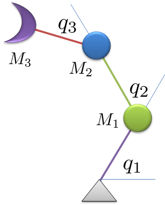
Let’s suppose a three DOF arm manipulator shown in the below figure. I am assuming all of masses (M1, M2, M3) exist at the end of links for simplicity. Three actuators exist at each joint, and directly actuate the torques (u1,u2,u3). The manipulator kinematics is governed by three joint angles (q1, q2, q3).

three DOF arm manipulator

2. Theoretical Background

We will get a dynamic equation of this system by using Lagrangian mechanics. If you do not have a background knowledge of Lagrangian mechanics, please refer here.

The general dynamic equation is obtained by

$\frac{d}{dt}\left( \frac{\partial T}{\partial \dot{q}_j}\right ) - \frac{\partial T}{\partial q_j} + \frac{\partial V}{\partial q_j} = P_j$

Where, T is the total kinetic energy, V is the total potential energy of the system. where $P_j$ is the generalized force, t is time, $q_j$ is the generalized coordinates, $\dot{q}_j$ is the generalized velocity. For the example of three-DOF arm manipulator problem, $P_j$ is the torque at the j-th joint, $q_j$ is the angle of the j-th joint, $\dot{q}_j$ is the angular velocity of the j-th joint.

3. Using Matlab symbolic toolbox

First, let’s define the symbols.

I am using x to represent q, xd for $\dot{q}$ , xdd for $\ddot{q}$ L is the length of each link. u is the torque of each joint. g is the gravity constant.

syms M1 M2 M3;
syms x1 x1d x1dd x2 x2d x2dd x3 x3d x3dd;
syms L1 L2 L3;
syms u1 u2 u3;
syms g

Second, find the position and velocities of the point masses.

p1x = L1cos(x1);
p1y = L1sin(x1);
p2x = p1x+L2cos(x1+x2);
p2y = p1y+L2sin(x1+x2);
p3x = p2x+L3cos(x1+x2+x3);
p3y = p2y+L3sin(x1+x2+x3);

v1x = -L1sin(x1)x1d;
v1y = +L1cos(x1)x1d;
v2x = v1x-L2sin(x1+x2)(x1d+x2d);
v2y = v1y+L2cos(x1+x2)(x1d+x2d);
v3x = v2x – L3sin(x1+x2+x3)(x1d+x2d+x3d);
v3y = v2y + L3cos(x1+x2+x3)(x1d+x2d+x3d);

Third, define the kinetic energy, and the potential energy.

KE = 0.5M1( v1x^2 + v1y^2) + 0.5M2( v2x^2 + v2y^2) + 0.5M3( v3x^2 + v3y^2);
KE = simplify(KE);

PE = M1gp1y + M2gp2y + M3gp3y;
PE = simplify(PE);

Fourth, define the generalized forces, here torques.

Px1 = u1;
Px2 = u2;
Px3 = u3;

Fifth, solve the Lagrangian equation

We have to get the Lagrangian eqn. $\frac{d}{dt}\left( \frac{\partial T}{\partial \dot{q}_j}\right ) - \frac{\partial T}{\partial q_j} + \frac{\partial V}{\partial q_j} = P_j$

Let’s obtain step by step.

$\left( \frac{\partial T}{\partial \dot{q}}\right )$ is obtained by

pKEpx1d = diff(KE,x1d);

To calculate, $\frac{d}{dt}\left( \frac{\partial T}{\partial \dot{q}}\right )$ , we need the chain rule, that is $\frac{d}{dt}\left( \frac{\partial T}{\partial \dot{q}_j}\right )= \sum^{3}_i \left\{ \frac{\partial }{\partial {q}_i}\left( \frac{\partial T}{\partial \dot{q}_j}\right )\frac{dq_i}{dt} + \frac{\partial }{\partial \dot{q}_i}\left( \frac{\partial T}{\partial {q}_j}\right )\frac{d \dot{q}_i}{dt} \right\}$

ddtpKEpx1d = diff(pKEpx1d,x1)x1d+ …
diff(pKEpx1d,x1d)x1dd+ …
diff(pKEpx1d,x2)x2d + …
diff(pKEpx1d,x2d)x2dd + …
diff(pKEpx1d,x3)x3d + …
diff(pKEpx1d,x3d)x3dd;

$\frac{\partial T}{\partial q_j}, \frac{\partial V}{\partial q_j}$ are easily obtained by

pKEpx1 = diff(KE,x1);
pPEpx1 = diff(PE,x1);

By summing all equations,

eqx1 = simplify( ddtpKEpx1d – pKEpx1 + pPEpx1 – Px1);

By repeating these procedures, we can get all governing equations.

Sixth, rearrange the equations.

We love more simplified forms like

$\frac{d}{dt} \begin{bmatrix} x_1\\ \dot{x}_1\\ x_2\\ \dot{x}_2\\ x_3\\ \dot{x}_3 \end{bmatrix}= f(x_1,\dot{x}_1,x_2,\dot{x}_2,x_3,\dot{x}_3)$

For this form, we need to rearrange the equations by

Sol = solve(eqx1,eqx2,eqx3,’x1dd,x2dd,x3dd’);
Sol.x1dd = simplify(Sol.x1dd);
Sol.x2dd = simplify(Sol.x2dd);
Sol.x3dd = simplify(Sol.x3dd);

Seventh, substitute with y1,y2… variables.

Just for easier implementation of symbolic codes, let’s substitute x1, x1d, x2, … with y1,y2….

syms y1 y2 y3 y4 y5 y6
fx1=subs(Sol.x1dd,{x1,x1d,x2,x2d,x3,x3d},{y1,y2,y3,y4,y5,y6})
fx2=subs(Sol.x2dd,{x1,x1d,x2,x2d,x3,x3d},{y1,y2,y3,y4,y5,y6})
fx3=subs(Sol.x3dd,{x1,x1d,x2,x2d,x3,x3d},{y1,y2,y3,y4,y5,y6})

Eighth, this is the result…. as you can see, it is almost impossible to solve by hand

fx1 =

(L2L3M2u1 – L2L3M2u2 + L2L3M3u1 – L2L3M3u2 – L1L3M2u2cos(y3) + L1L3M2u3cos(y3) – L1L3M3u2cos(y3) + L1L3M3u3cos(y3) – L2L3M3u1cos(y5)^2 + L2L3M3u2cos(y5)^2 + L1L2^2L3M2^2y2^2sin(y3) + L1L2^2L3M2^2y4^2sin(y3) – L1L2L3M2^2gcos(y1) + (L1^2L2L3M2^2y2^2sin(2y3))/2 + L1L2M2u3sin(y3)sin(y5) + L1L2M3u3sin(y3)sin(y5) + L1L3M3u2cos(y3)cos(y5)^2 – L1L3M3u3cos(y3)cos(y5)^2 + L1L2^2L3M2M3y2^2sin(y3) + L1L2^2L3M2M3y4^2sin(y3) – L1L2L3M1M2gcos(y1) – L1L2L3M1M3gcos(y1) – L1L2L3M2M3gcos(y1) + 2L1L2^2L3M2^2y2y4sin(y3) + (L1^2L2L3M2M3y2^2sin(2y3))/2 – L1L3M3u2cos(y5)sin(y3)sin(y5) + L1L3M3u3cos(y5)sin(y3)sin(y5) + L1L2L3M2^2gcos(y1)cos(y3)^2 – L1L2L3M2^2gcos(y3)sin(y1)sin(y3) + 2L1L2^2L3M2M3y2y4sin(y3) + L1L2L3M2M3gcos(y1)cos(y3)^2 + L1L2L3M1M3gcos(y1)cos(y5)^2 + L1L2L3^2M2M3y2^2cos(y5)sin(y3) + L1L2L3^2M2M3y4^2cos(y5)sin(y3) + L1L2L3^2M2M3y6^2cos(y5)sin(y3) + 2L1L2L3^2M2M3y2y4cos(y5)sin(y3) + 2L1L2L3^2M2M3y2y6cos(y5)sin(y3) + 2L1L2L3^2M2M3y4y6cos(y5)sin(y3) – L1L2L3M2M3gcos(y3)sin(y1)sin(y3))/(L1^2L2L3(M2^2 – M2^2cos(y3)^2 + M1M2 + M1M3 + M2M3 – M2M3cos(y3)^2 – M1M3*cos(y5)^2))

fx2 =

-(2L1^2L3M1u3 – 2L1^2L3M1u2 – 2L1^2L3M2u2 + 2L2^2L3M2u1 + 2L1^2L3M2u3 – L1^2L3M3u2 – 2L2^2L3M2u2 + L2^2L3M3u1 + L1^2L3M3u3 – L2^2L3M3u2 + L1L2^2M2u3cos(y3 – y5) + L1L2^2M3u3cos(y3 – y5) – L1^2L2M2u3cos(2y3 + y5) – L1^2L2M3u3cos(2y3 + y5) – L2^2L3M3u1cos(2y5) + L2^2L3M3u2cos(2y5) + L1^2L3M3u2cos(2y3 + 2y5) – L1^2L3M3u3cos(2y3 + 2y5) – L1L2^2M2u3cos(y3 + y5) – L1L2^2M3u3cos(y3 + y5) + 2L1^2L2M1u3cos(y5) + L1^2L2M2u3cos(y5) + L1^2L2M3u3cos(y5) + 2L1L2^3L3M2^2y2^2sin(y3) + 2L1^3L2L3M2^2y2^2sin(y3) + 2L1L2^3L3M2^2y4^2sin(y3) – L1L2L3M3u1cos(y3 + 2y5) + 2L1L2L3M3u2cos(y3 + 2y5) – L1L2L3M3u3cos(y3 + 2y5) + L1^2L2L3M2^2gcos(y1 + y3) – L1L2^2L3M2^2gcos(y1) – L1^2L2L3M2^2gcos(y1 – y3) + L1L2^2L3M2^2gcos(y1 + 2y3) + 2L1^2L2^2L3M2^2y2^2sin(2y3) + L1^2L2^2L3M2^2y4^2sin(2y3) + 2L1L2L3M2u1cos(y3) – 4L1L2L3M2u2cos(y3) + L1L2L3M3u1cos(y3) + 2L1L2L3M2u3cos(y3) – 2L1L2L3M3u2cos(y3) + L1L2L3M3u3cos(y3) + 2L1^3L2L3M1M2y2^2sin(y3) + L1^3L2L3M1M3y2^2sin(y3) + 2L1L2^3L3M2M3y2^2sin(y3) + 2L1^3L2L3M2M3y2^2sin(y3) + 2L1L2^3L3M2M3y4^2sin(y3) + 4L1L2^3L3M2^2y2y4sin(y3) – (L1^2L2L3M1M3gcos(y1 + y3 + 2y5))/2 – L1^3L2L3M1M3y2^2sin(y3 + 2y5) + L1L2^2L3^2M2M3y2^2sin(y3 + y5) + L1L2^2L3^2M2M3y4^2sin(y3 + y5) + L1L2^2L3^2M2M3y6^2sin(y3 + y5) + L1^2L2L3M1M2gcos(y1 + y3) + (L1^2L2L3M1M3gcos(y1 + y3))/2 + L1^2L2L3M2M3gcos(y1 + y3) – 2L1^2L2L3^2M1M3y2^2sin(y5) – L1^2L2L3^2M2M3y2^2sin(y5) – 2L1^2L2L3^2M1M3y4^2sin(y5) – L1^2L2L3^2M2M3y4^2sin(y5) – 2L1^2L2L3^2M1M3y6^2sin(y5) – L1^2L2L3^2M2M3y6^2sin(y5) – 2L1L2^2L3M1M2gcos(y1) – L1L2^2L3M1M3gcos(y1) – L1L2^2L3M2M3gcos(y1) + (L1^2L2L3M1M3gcos(y1 – y3 – 2y5))/2 + L1L2^2L3^2M2M3y2^2sin(y3 – y5) + L1^2L2L3^2M2M3y2^2sin(2y3 + y5) + L1L2^2L3^2M2M3y4^2sin(y3 – y5) + L1^2L2L3^2M2M3y4^2sin(2y3 + y5) + L1L2^2L3^2M2M3y6^2sin(y3 – y5) + L1^2L2L3^2M2M3y6^2sin(2y3 + y5) – L1^2L2L3M1M2gcos(y1 – y3) – (L1^2L2L3M1M3gcos(y1 – y3))/2 – L1^2L2L3M2M3gcos(y1 – y3) + L1L2^2L3M2M3gcos(y1 + 2y3) + (L1L2^2L3M1M3gcos(y1 – 2y5))/2 + (L1L2^2L3M1M3gcos(y1 + 2y5))/2 + 2L1^2L2^2L3M2M3y2^2sin(2y3) – L1^2L2^2L3M1M3y2^2sin(2y5) + L1^2L2^2L3M2M3y4^2sin(2y3) – L1^2L2^2L3M1M3y4^2sin(2y5) + 2L1^2L2^2L3M2^2y2y4sin(2y3) + 4L1L2^3L3M2M3y2y4sin(y3) + 2L1L2^2L3^2M2M3y2y4sin(y3 + y5) + 2L1L2^2L3^2M2M3y2y6sin(y3 + y5) + 2L1L2^2L3^2M2M3y4y6sin(y3 + y5) – 4L1^2L2L3^2M1M3y2y4sin(y5) – 2L1^2L2L3^2M2M3y2y4sin(y5) – 4L1^2L2L3^2M1M3y2y6sin(y5) – 2L1^2L2L3^2M2M3y2y6sin(y5) – 4L1^2L2L3^2M1M3y4y6sin(y5) – 2L1^2L2L3^2M2M3y4y6sin(y5) + 2L1L2^2L3^2M2M3y2y4sin(y3 – y5) + 2L1^2L2L3^2M2M3y2y4sin(2y3 + y5) + 2L1L2^2L3^2M2M3y2y6sin(y3 – y5) + 2L1^2L2L3^2M2M3y2y6sin(2y3 + y5) + 2L1L2^2L3^2M2M3y4y6sin(y3 – y5) + 2L1^2L2L3^2M2M3y4y6sin(2y3 + y5) + 2L1^2L2^2L3M2M3y2y4sin(2y3) – 2L1^2L2^2L3M1M3y2y4sin(2y5))/(L1^2L2^2L3(M2^2 – M2^2cos(2y3) + 2M1M2 + M1M3 + M2M3 – M2M3cos(2y3) – M1M3cos(2*y5)))

fx3 =

-(L1L3^2M3^2u2 – L1L2^2M3^2u3 – L1L2^2M2^2u3 – L1L3^2M3^2u3 – L2L3^2M3^2u1cos(y3) + L2L3^2M3^2u2cos(y3) – 2L1L2^2M1M2u3 – 2L1L2^2M1M3u3 + 2L1L3^2M1M3u2 – 2L1L2^2M2M3u3 – 2L1L3^2M1M3u3 + 2L1L3^2M2M3u2 – 2L1L3^2M2M3u3 + L1L2^2M2^2u3cos(2y3) + L1L2^2M3^2u3cos(2y3) + L1L3^2M3^2u2sin(2y3)sin(2y5) – L1L3^2M3^2u3sin(2y3)sin(2y5) + L1L2L3M3^2u2cos(y5) – 2L1L2L3M3^2u3cos(y5) – 2L2L3^2M2M3u1cos(y3) + 2L2L3^2M2M3u2cos(y3) – 2L2^2L3M3^2u1sin(y3)sin(y5) + 2L2^2L3M3^2u2sin(y3)sin(y5) + L2L3^2M3^2u1cos(2y5)cos(y3) – L2L3^2M3^2u2cos(2y5)cos(y3) + 2L1L2^2M2M3u3cos(2y3) – L2L3^2M3^2u1sin(2y5)sin(y3) + L2L3^2M3^2u2sin(2y5)sin(y3) – L1L3^2M3^2u2cos(2y3)cos(2y5) + L1L3^2M3^2u3cos(2y3)cos(2y5) – L1L2^2L3^2M2M3^2y2^2sin(2y3) – L1L2^2L3^2M2^2M3y2^2sin(2y3) + 2L1L2^2L3^2M1M3^2y2^2sin(2y5) – L1L2^2L3^2M2M3^2y4^2sin(2y3) – L1L2^2L3^2M2^2M3y4^2sin(2y3) + 2L1L2^2L3^2M1M3^2y4^2sin(2y5) + L1L2^2L3^2M1M3^2y6^2sin(2y5) + 2L1L2L3M1M3u2cos(y5) – 4L1L2L3M1M3u3cos(y5) + L1L2L3M2M3u2cos(y5) – 2L1L2L3M2M3u3cos(y5) – 2L2^2L3M2M3u1sin(y3)sin(y5) + 2L2^2L3M2M3u2sin(y3)sin(y5) + 2L1L2L3^3M1M3^2y2^2sin(y5) + 2L1L2^3L3M1M3^2y2^2sin(y5) + L1L2L3^3M2M3^2y2^2sin(y5) + 2L1L2L3^3M1M3^2y4^2sin(y5) + 2L1L2^3L3M1M3^2y4^2sin(y5) + L1L2L3^3M2M3^2y4^2sin(y5) + 2L1L2L3^3M1M3^2y6^2sin(y5) + L1L2L3^3M2M3^2y6^2sin(y5) – L1L2L3M3^2u2cos(2y3)cos(y5) + 2L1L2L3M3^2u3cos(2y3)cos(y5) + L1L2L3M3^2u2sin(2y3)sin(y5) – 2L1L2L3M3^2u3sin(2y3)sin(y5) – L1^2L2L3^2M1M3^2y2^2sin(y3) – 2L1^2L2L3^2M2M3^2y2^2sin(y3) – 2L1^2L2L3^2M2^2M3y2^2sin(y3) – 2L1L2^2L3^2M2M3^2y2y4sin(2y3) – 2L1L2^2L3^2M2^2M3y2y4sin(2y3) + 4L1L2^2L3^2M1M3^2y2y4sin(2y5) + 2L1L2^2L3^2M1M3^2y2y6sin(2y5) + 2L1L2^2L3^2M1M3^2y4y6sin(2y5) + 2L1L2^3L3M1M2M3y2^2sin(y5) + 2L1L2^3L3M1M2M3y4^2sin(y5) – L1L2L3M2M3u2cos(2y3)cos(y5) + 2L1L2L3M2M3u3cos(2y3)cos(y5) + 4L1L2L3^3M1M3^2y2y4sin(y5) + 4L1L2^3L3M1M3^2y2y4sin(y5) + 2L1L2L3^3M2M3^2y2y4sin(y5) + 4L1L2L3^3M1M3^2y2y6sin(y5) + 2L1L2L3^3M2M3^2y2y6sin(y5) + 4L1L2L3^3M1M3^2y4y6sin(y5) + 2L1L2L3^3M2M3^2y4y6sin(y5) + L1L2L3M2M3u2sin(2y3)sin(y5) – 2L1L2L3M2M3u3sin(2y3)sin(y5) – L1L2L3^3M2M3^2y2^2cos(2y3)sin(y5) – L1L2L3^3M2M3^2y2^2sin(2y3)cos(y5) – L1L2L3^3M2M3^2y4^2cos(2y3)sin(y5) – L1L2L3^3M2M3^2y4^2sin(2y3)cos(y5) – L1L2L3^3M2M3^2y6^2cos(2y3)sin(y5) – L1L2L3^3M2M3^2y6^2sin(2y3)cos(y5) + 2L1^2L2^2L3M1M3^2y2^2cos(y3)sin(y5) – 2L1^2L2L3^2M1M2M3y2^2sin(y3) + L1L2L3^2M1M3^2gsin(y1)sin(y3) + 2L1L2L3^2M2M3^2gsin(y1)sin(y3) + 2L1L2L3^2M2^2M3gsin(y1)sin(y3) + L1^2L2L3^2M1M3^2y2^2cos(2y5)sin(y3) + L1^2L2L3^2M1M3^2y2^2sin(2y5)cos(y3) – L1L2L3^2M1M3^2gcos(2y5)sin(y1)sin(y3) – L1L2L3^2M1M3^2gsin(2y5)cos(y3)sin(y1) + 4L1L2^3L3M1M2M3y2y4sin(y5) + 2L1^2L2^2L3M1M2M3y2^2cos(y3)sin(y5) – 2L1L2L3^3M2M3^2y2y4cos(2y3)sin(y5) – 2L1L2L3^3M2M3^2y2y4sin(2y3)cos(y5) – 2L1L2L3^3M2M3^2y2y6cos(2y3)sin(y5) – 2L1L2L3^3M2M3^2y2y6sin(2y3)cos(y5) – 2L1L2L3^3M2M3^2y4y6cos(2y3)sin(y5) – 2L1L2L3^3M2M3^2y4y6sin(2y3)cos(y5) – 2L1L2^2L3M1M3^2gcos(y3)sin(y1)sin(y5) + 2L1L2L3^2M1M2M3gsin(y1)sin(y3) – 2L1L2^2L3M1M2M3gcos(y3)sin(y1)sin(y5))/(L1L2^2L3^2M3(M2^2 – M2^2cos(2y3) + 2M1M2 + M1M3 + M2M3 – M2M3cos(2y3) – M1M3cos(2y5)))

4. Now it is ready!!! let’s run a simulation!

copy the result and paste the symbols in a Matlab function. Then, run an ODE with the function.

A sample code is here.

<Download>

In the attached file, “Symb_Development_3DOF.m” generates a dynamic model. “main_sim_three_dof_arm.m” runs a simulation. Then, you can get this result.

So far, I have explained how to derive a Lagrange Equation by MATLAB with Examples. I hope that this post helps your project and save your time. Please leave a message if you have any question.

Update on 02/21/2016

I updated some code and posting about typo. “simple” -> “simplify” There is no function “simple” Now all programs are running well.

-Mok-

Reference

[1] http://en.wikipedia.org/wiki/Lagrangian_mechanics

[2] https://www.google.com/url?sa=t&rct=j&q=&esrc=s&source=web&cd=1&ved=0CB8QFjAA&url=http%3A%2F%2Fsstl.cee.illinois.edu%2Fapss%2Ffiles%2FLagrange_Reference.doc&ei=iF9SVYT0N8TJtQXCwoDgCQ&usg=AFQjCNEyv1Ut3cGu6ylAjtZyG6ZPCYQkIg&sig2=pJ-84gdkjCqH_AH9pB6tjA&bvm=bv.92885102,d.b2w&cad=rja

[3] http://www.mathworks.com/matlabcentral/fileexchange/23037-lagrange-s-equations

[4] https://www.google.com/url?sa=t&rct=j&q=&esrc=s&source=web&cd=4&cad=rja&uact=8&ved=0CDIQFjAD&url=http%3A%2F%2Fweb.stanford.edu%2Fclass%2Fme328%2Flectures%2Flecture6-dynamics.pdf&ei=oJ5kVa7CG4GKsQWDloFQ&usg=AFQjCNGWFZZ4uBP_ObHHnirkEzAIc5OONw&sig2=ISnRQj-kBc0y_eoT_0y7Hw&bvm=bv.93990622,d.b2w

Accurate, Robust, and Real-time Estimation of Finger Pose with a Motion Capture System

Leave a reply

Finger exoskeletons and haptic devices demand an accurate, robust, and fast estimation of finger pose. We present a novel finger pose estimation method using a motion capture system. The method combines system identification and state estimation in a unified framework. The system identification stage investigates the accurate model of a finger, and the state estimation stage tracks the finger pose with Extended Kalman Filter (EKF) algorithm based on the model obtained in the system identification stage. The algorithm is validated by simulation and experiment. The experiment results show that the method can estimate the finger pose faster than 1 Khz and robustly against the measurement noise, occlusion of markers, and fast movement.

Sorry, no publications matched your criteria.

Previous research

Leave a reply

>> 3D Environment Reconstruction & 3D SLAM based on Plane Feature

– Period : September, 2010 ~ 2012

– Co-research with Prof. Nakju Doh, and Sooyong Yeon, Robotics Lab., Korea University
– Feature-based 3D SLAM(Simultaneous Localization and Mapping) algorithms can overcome weak points of non-feature-based (point-based) 3D SLAM algorithm such as ICP. Plane feature-based 3D SLAM approach manages map with plane features, which enables 3D SLAM at large-scale environment in real time.

* click to see a large picture

– Related Papers:

Sooyong Yeon, Changhyun Jun, Hyunga Choi, Jaehyeon Kang, Youngmok Yun, and Nakju Lett Doh, “Robust-PCA based Hierarchical Plane Extraction for the Application of Geometric 3D SLAM,” Industrial Robot, in Press

>> Outdoor Multi-robot Formation Control

– Period : July, 2011 ~
– Project of Agency for Defense Development(ADD), directed by Dr. Changhwan Kim, Korea Institute of Science and Technology(KIST)
– The goal of this project is first to control outdoor multi-robot with particular formations. Additionally, this control algorithm will be fused with other various applications such as surveillance, and invader searching.

– Application : Cooperative Control For Optimal Surveillance

YouTube 동영상

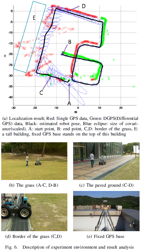
>> Outdoor Localization with Optical Navigation Sensor, IMU and GPS

Autonomous outdoor navigation algorithms are required in various military and industry fields. A stable and robust outdoor localization algorithm is critical to successful outdoor
navigation. However, unpredictable external effects and interruption of the GPS signal cause difficulties in outdoor localization. To address this issue, first we devised a new optical navigation
sensor that measures a mobile robot’s transverse distance without being subjected to external influence. Next, using the optical navigation sensor, a novel localization algorithm is established with Inertial-Measurement-Unit (IMU) and GPS. The algorithm is verified in an urban environment where the GPS signal is frequently interrupted and rough ground surfaces provide serious disturbances.

– Related Papers:

Youngmok Yun, Jingfu Jin, Namhoon Kim, Jeongyeon Yoon, and Changhwan Kim, “Outdoor localization with optical navigation sensor, IMU and GPS,” Int. Conf. on Multisensor Fusion and Integration for Intelligent Systems (MFI), pp. 377-382. IEEE, 2012.

>> Mechatronic System Design and Control for Automobile System Validation

– Period : April, 2008 ~ June, 2011

– Assistant Researcher, Renault-Samsung Motors Technical Center
– As a military service, for three years, I had worked at the Renault-Samsung Motors Technical Center. Main tasks were mechatronic system design and control for validation of automobile chassis system. Through these experience, I could learn about the practical design sense of mechanical and electronic system. Additionally, global cooperation with world-wide coworkers and participation to several huge-scale automobile projects were another pleasure.

< Steering Performance Test Bench >

< Acc., Brake, Clutch Pedal & Parking Brake Durability Test Bench >

>> Odometry Calibration of Mobile Robot using Home-positioning

– Period : 2007

– Advisor : Prof. Wankyun Chung, Robotics Lab., POSTECH

– The subject of MS graduation thesis was “Odometry calibration of mobile robot using home-positioning.” Home-positioning frequently occurs due to the reason of recharge or initialization of mobile robot. What is even better is that its technique is maturely developed and already adopted in many commercial robots. My ideas was that home-positioning can be used as a powerful measurement of mobile robot, and this would lead high accuracy of odometry. You may see the detail idea at the below poster.

– Related Papers:

– Youngmok Yun, Byungjae Park, and Wan Kyun Chung, “Odometry Calibration using Home Positioning Function for Mobile Robot,” IEEE Int. Conf. on Robotics and Automation (ICRA), 2008.

– Sharifuddin Mondal, Youngmok Yun, and Wan Kyun Chung, “Terminal Iterative Learning Control for Calibrating Systematic Odometry Errors in Mobile Robots,” IEEE/ASME Int. Conf. on Advanced Intelligent Mechatronics (AIM), 2010.

– Youngmok Yun, Wan Kyun Chung, and Sang yep Nam, “Systematic Error Calibration of Mobile Robot using Home Positioning Function,” IEEE Int. Conf. on Ubiquitous Robots and Ambient Intelligence (URAI), 2008.

>> Development of Navigation and Human-robot Interaction Techniques

– Period : 2006 ~ 2007

– Director : Prof. Wankyun Chung, Robotics Lab., POSTECH

– Project of Korean Ministry of Information and Communication

– Mobile robot team, Robotics Lab, POSTECH, developed autonomous mobile robot framework including SLAM, exploration, and path-planning. I took part in SLAM algorithm development and visual-feature recognition.

SLAM movie clip, Robotics Lab, POSTECH

>> Tennis ball gathering robot using visual recognition

– Period : 2004 ~ 2005

– Graduation project, Mechanical Engineering Dept., POSTECH

– Winner of the graduation project.

– As a graduation project of ME, POSTECH, our team made tennis ball gathering robot using visual recognition. The task of the robot was to gather all tennis balls in a room. Frankly, now I can know that it was too difficult subject for undergraduate students to build all system and programs only within one year because there were too many things to do: mechanical design, electronic system organization, visual recognition programming, navigation algorithm programming and others. However, we devoted ourselves to the project, and finally, we won the competition of the project.

Statistical Method for Prediction of Human Walking Pattern with Gaussian Process Regression

Leave a reply

Statistical Method for Prediction of Human Walking Pattern with Gaussian Process Regression

We propose a novel methodology for predicting human gait pattern kinematics based on a statistical and stochastic approach using a method called Gaussian process regression (GPR). We selected 14 body parameters that significantly affect the gait pattern and 14 joint motions that represent gait kinematics. The body parameter and gait kinematics data were recorded from 113 subjects by anthropometric measurements and a motion capture system. We generated a regression model with GPR for gait pattern prediction and built a stochastic function mapping from body parameters to gait kinematics based on the database and GPR, and validated the model with a cross validation method. The function can not only produce trajectories for the joint motions associated with gait kinematics, but can also estimate the associated uncertainties. Our approach results in a novel, low-cost and subject-specific method for predicting gait kinematics with only the subject’s body parameters as the necessary input, and also enables a comprehensive understanding of the correlation and uncertainty between body parameters and gait kinematics.

Sorry, no publications matched your criteria.

Numerical Jacobian matrix calculation method with matlab code

20 Replies

In this post, I share a numerical Jacobian matrix calculation method with matlab code.

Actually there is a function in Matlab inherently, but it is very complex. ( look at the function, NumJac ), So I made a very simple version. I wish this can help you.

You can download from here.

The attachment file includes

1. NumJacob.m : main file it generates jacobian matrix.

2. Demo.m : demo file

3. test_func.m : test function to show its demo

The below is a simple example.

>> NumJacob(@cos,1)

ans =

-0.8415

>> x0=[0;1]; other_param=[1;2];
>> df=NumJacob(@test_func,x0,other_param)

df =

1.0000 0
0 2.0000

Because the code is very easy, probably you can easily understand the codes.

Then, good luck ^^

if you have any question, please leave me a comment below.

Added on Feb 07. 2014

I am uploading another demo file to give a solution of Mahmudul’s request (for detail, see the comment).

This demo file is to get a numerical Jacobian for the below function

y1′ = y2*y3; y1(0) = 0
y2′ = -y1*y3; y2(0) = 1
y3′ = -0.51*y1*y3; y3(0) =1

Download this demo file.

Added on Mar/21 2015

If you are interested in calculating numerical Jocobian matrix for a complex number, please read this post.

http://youngmok.com/matlab-code-for-numerical-calculation-of-jacobian-matrix-for-a-complex-number/

—————————————————————————————————

I am Youngmok Yun, and writing about robotics theories and my research.

My main site is http://youngmok.com, and Korean ver. is http://yunyoungmok.tistory.com.

—————————————————————————————————

Parallel computation with Matlab, SPMD. Explanation with simple example code

2 Replies

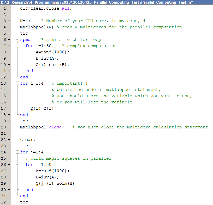
Today I’d like to introduce a parallel computation skill in Matlab.

I also heard that the use of parallel computation in Matlab is very easy. But it was better than my expectation. Wonderful!!

You need to know the usage of SPMD. It is pretty easy.

First let’s the code, you can also download this file in the attachment, click <here>.

The result is the below

Starting matlabpool using the ‘local’ configuration … connected to 4 labs.
Elapsed time is 120.482356 seconds.
Sending a stop signal to all the labs … stopped.
Elapsed time is 167.796932 seconds.

Because, I did many other works in the calculation time, Its result is not very fast, The slowest CPU core determined the final computation time. But its performance is really good if you have more than 4 multi cpu cores.

I wish this post can help your understanding about the use of SPMD in Matlab.

if you have any question, please leave me a comment below.

—————————————————————————————————

I am Youngmok Yun, and writing about robotics theories and my research.

My main site is http://youngmok.com, and Korean ver. is http://yunyoungmok.tistory.com.

—————————————————————————————————

Youngmok Yun: Roboticist in Austin

Category Archives: Research

Vertex angle from three points, Matlab code

Like this:

Lagrange Equation by MATLAB with Examples

Lagrange Equation by MATLAB with Examples

1. Example system

2. Theoretical Background