Tag Archives: matlab

Matlab Code for Numerical Hessian Matrix

2 Replies

Matlab code for numerical hessian matrix

In this post, I am sharing a Malab code calculating a numerical hessian matrix.

You can download here.

You can use NumHessian.m with this syntax.

function hf = NumHessian(f,x0,varargin)

You can understand how to use simply by reading these two simple examples.

Example 1

>> NumHessian(@cos,0)

ans =

-1.0000

Example 2

function y=test_func(x,a)
y=ax(1)x(2)*x(3);

>> NumHessian(@test_func,[1 2 3]’,2)

ans =

0 6.0000 4.0000
5.9999 -0.0001 1.9998
3.9999 2.0000 0

I hope this Matlab code for numerical Hessian matrix helps your projects

This Matlab code is based on another Matlab function, NumJacob, which calculates a numerical Jacobian matrix. If you are interested in this, visit here.

If you want to know the theory on Hessian matrix, please read this Wiki.

I acknowledge that this code is originally made by Parviz Khavari, a visitor of this blog, and I modified to post here.

Vertex angle from three points, Matlab code

Lagrange Equation by MATLAB with Examples

12 Replies

Lagrange Equation by MATLAB with Examples

In this post, I will explain how to derive a dynamic equation with Lagrange Equation by MATLAB with Examples. As an example, I will derive a dynamic model of a three-DOF arm manipulator (or triple pendulum). Of course you may get a dynamic model for a two-DOF arm manipulator by simply removing several lines. I am attaching demo codes for both two and three DOF arm manipulators.

If you know all theories and necessary skills and if you just want source code, you can just download from here.

<Download>

In the attached file, “Symb_Development_3DOF.m” generates a dynamic model. “main_sim_three_dof_arm.m” runs a simulation. You may get a result like this.

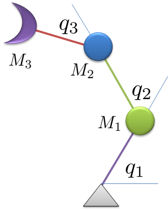
1. Example system

Let’s suppose a three DOF arm manipulator shown in the below figure. I am assuming all of masses (M1, M2, M3) exist at the end of links for simplicity. Three actuators exist at each joint, and directly actuate the torques (u1,u2,u3). The manipulator kinematics is governed by three joint angles (q1, q2, q3).

three DOF arm manipulator

2. Theoretical Background

We will get a dynamic equation of this system by using Lagrangian mechanics. If you do not have a background knowledge of Lagrangian mechanics, please refer here.

The general dynamic equation is obtained by

$\frac{d}{dt}\left( \frac{\partial T}{\partial \dot{q}_j}\right ) - \frac{\partial T}{\partial q_j} + \frac{\partial V}{\partial q_j} = P_j$

Where, T is the total kinetic energy, V is the total potential energy of the system. where $P_j$ is the generalized force, t is time, $q_j$ is the generalized coordinates, $\dot{q}_j$ is the generalized velocity. For the example of three-DOF arm manipulator problem, $P_j$ is the torque at the j-th joint, $q_j$ is the angle of the j-th joint, $\dot{q}_j$ is the angular velocity of the j-th joint.

3. Using Matlab symbolic toolbox

First, let’s define the symbols.

I am using x to represent q, xd for $\dot{q}$ , xdd for $\ddot{q}$ L is the length of each link. u is the torque of each joint. g is the gravity constant.

syms M1 M2 M3;
syms x1 x1d x1dd x2 x2d x2dd x3 x3d x3dd;
syms L1 L2 L3;
syms u1 u2 u3;
syms g

Second, find the position and velocities of the point masses.

p1x = L1cos(x1);
p1y = L1sin(x1);
p2x = p1x+L2cos(x1+x2);
p2y = p1y+L2sin(x1+x2);
p3x = p2x+L3cos(x1+x2+x3);
p3y = p2y+L3sin(x1+x2+x3);

v1x = -L1sin(x1)x1d;
v1y = +L1cos(x1)x1d;
v2x = v1x-L2sin(x1+x2)(x1d+x2d);
v2y = v1y+L2cos(x1+x2)(x1d+x2d);
v3x = v2x – L3sin(x1+x2+x3)(x1d+x2d+x3d);
v3y = v2y + L3cos(x1+x2+x3)(x1d+x2d+x3d);

Third, define the kinetic energy, and the potential energy.

KE = 0.5M1( v1x^2 + v1y^2) + 0.5M2( v2x^2 + v2y^2) + 0.5M3( v3x^2 + v3y^2);
KE = simplify(KE);

PE = M1gp1y + M2gp2y + M3gp3y;
PE = simplify(PE);

Fourth, define the generalized forces, here torques.

Px1 = u1;
Px2 = u2;
Px3 = u3;

Fifth, solve the Lagrangian equation

We have to get the Lagrangian eqn. $\frac{d}{dt}\left( \frac{\partial T}{\partial \dot{q}_j}\right ) - \frac{\partial T}{\partial q_j} + \frac{\partial V}{\partial q_j} = P_j$

Let’s obtain step by step.

$\left( \frac{\partial T}{\partial \dot{q}}\right )$ is obtained by

pKEpx1d = diff(KE,x1d);

To calculate, $\frac{d}{dt}\left( \frac{\partial T}{\partial \dot{q}}\right )$ , we need the chain rule, that is $\frac{d}{dt}\left( \frac{\partial T}{\partial \dot{q}_j}\right )= \sum^{3}_i \left\{ \frac{\partial }{\partial {q}_i}\left( \frac{\partial T}{\partial \dot{q}_j}\right )\frac{dq_i}{dt} + \frac{\partial }{\partial \dot{q}_i}\left( \frac{\partial T}{\partial {q}_j}\right )\frac{d \dot{q}_i}{dt} \right\}$

ddtpKEpx1d = diff(pKEpx1d,x1)x1d+ …
diff(pKEpx1d,x1d)x1dd+ …
diff(pKEpx1d,x2)x2d + …
diff(pKEpx1d,x2d)x2dd + …
diff(pKEpx1d,x3)x3d + …
diff(pKEpx1d,x3d)x3dd;

$\frac{\partial T}{\partial q_j}, \frac{\partial V}{\partial q_j}$ are easily obtained by

pKEpx1 = diff(KE,x1);
pPEpx1 = diff(PE,x1);

By summing all equations,

eqx1 = simplify( ddtpKEpx1d – pKEpx1 + pPEpx1 – Px1);

By repeating these procedures, we can get all governing equations.

Sixth, rearrange the equations.

We love more simplified forms like

$\frac{d}{dt} \begin{bmatrix} x_1\\ \dot{x}_1\\ x_2\\ \dot{x}_2\\ x_3\\ \dot{x}_3 \end{bmatrix}= f(x_1,\dot{x}_1,x_2,\dot{x}_2,x_3,\dot{x}_3)$

For this form, we need to rearrange the equations by

Sol = solve(eqx1,eqx2,eqx3,’x1dd,x2dd,x3dd’);
Sol.x1dd = simplify(Sol.x1dd);
Sol.x2dd = simplify(Sol.x2dd);
Sol.x3dd = simplify(Sol.x3dd);

Seventh, substitute with y1,y2… variables.

Just for easier implementation of symbolic codes, let’s substitute x1, x1d, x2, … with y1,y2….

syms y1 y2 y3 y4 y5 y6
fx1=subs(Sol.x1dd,{x1,x1d,x2,x2d,x3,x3d},{y1,y2,y3,y4,y5,y6})
fx2=subs(Sol.x2dd,{x1,x1d,x2,x2d,x3,x3d},{y1,y2,y3,y4,y5,y6})
fx3=subs(Sol.x3dd,{x1,x1d,x2,x2d,x3,x3d},{y1,y2,y3,y4,y5,y6})

Eighth, this is the result…. as you can see, it is almost impossible to solve by hand

fx1 =

(L2L3M2u1 – L2L3M2u2 + L2L3M3u1 – L2L3M3u2 – L1L3M2u2cos(y3) + L1L3M2u3cos(y3) – L1L3M3u2cos(y3) + L1L3M3u3cos(y3) – L2L3M3u1cos(y5)^2 + L2L3M3u2cos(y5)^2 + L1L2^2L3M2^2y2^2sin(y3) + L1L2^2L3M2^2y4^2sin(y3) – L1L2L3M2^2gcos(y1) + (L1^2L2L3M2^2y2^2sin(2y3))/2 + L1L2M2u3sin(y3)sin(y5) + L1L2M3u3sin(y3)sin(y5) + L1L3M3u2cos(y3)cos(y5)^2 – L1L3M3u3cos(y3)cos(y5)^2 + L1L2^2L3M2M3y2^2sin(y3) + L1L2^2L3M2M3y4^2sin(y3) – L1L2L3M1M2gcos(y1) – L1L2L3M1M3gcos(y1) – L1L2L3M2M3gcos(y1) + 2L1L2^2L3M2^2y2y4sin(y3) + (L1^2L2L3M2M3y2^2sin(2y3))/2 – L1L3M3u2cos(y5)sin(y3)sin(y5) + L1L3M3u3cos(y5)sin(y3)sin(y5) + L1L2L3M2^2gcos(y1)cos(y3)^2 – L1L2L3M2^2gcos(y3)sin(y1)sin(y3) + 2L1L2^2L3M2M3y2y4sin(y3) + L1L2L3M2M3gcos(y1)cos(y3)^2 + L1L2L3M1M3gcos(y1)cos(y5)^2 + L1L2L3^2M2M3y2^2cos(y5)sin(y3) + L1L2L3^2M2M3y4^2cos(y5)sin(y3) + L1L2L3^2M2M3y6^2cos(y5)sin(y3) + 2L1L2L3^2M2M3y2y4cos(y5)sin(y3) + 2L1L2L3^2M2M3y2y6cos(y5)sin(y3) + 2L1L2L3^2M2M3y4y6cos(y5)sin(y3) – L1L2L3M2M3gcos(y3)sin(y1)sin(y3))/(L1^2L2L3(M2^2 – M2^2cos(y3)^2 + M1M2 + M1M3 + M2M3 – M2M3cos(y3)^2 – M1M3*cos(y5)^2))

fx2 =

-(2L1^2L3M1u3 – 2L1^2L3M1u2 – 2L1^2L3M2u2 + 2L2^2L3M2u1 + 2L1^2L3M2u3 – L1^2L3M3u2 – 2L2^2L3M2u2 + L2^2L3M3u1 + L1^2L3M3u3 – L2^2L3M3u2 + L1L2^2M2u3cos(y3 – y5) + L1L2^2M3u3cos(y3 – y5) – L1^2L2M2u3cos(2y3 + y5) – L1^2L2M3u3cos(2y3 + y5) – L2^2L3M3u1cos(2y5) + L2^2L3M3u2cos(2y5) + L1^2L3M3u2cos(2y3 + 2y5) – L1^2L3M3u3cos(2y3 + 2y5) – L1L2^2M2u3cos(y3 + y5) – L1L2^2M3u3cos(y3 + y5) + 2L1^2L2M1u3cos(y5) + L1^2L2M2u3cos(y5) + L1^2L2M3u3cos(y5) + 2L1L2^3L3M2^2y2^2sin(y3) + 2L1^3L2L3M2^2y2^2sin(y3) + 2L1L2^3L3M2^2y4^2sin(y3) – L1L2L3M3u1cos(y3 + 2y5) + 2L1L2L3M3u2cos(y3 + 2y5) – L1L2L3M3u3cos(y3 + 2y5) + L1^2L2L3M2^2gcos(y1 + y3) – L1L2^2L3M2^2gcos(y1) – L1^2L2L3M2^2gcos(y1 – y3) + L1L2^2L3M2^2gcos(y1 + 2y3) + 2L1^2L2^2L3M2^2y2^2sin(2y3) + L1^2L2^2L3M2^2y4^2sin(2y3) + 2L1L2L3M2u1cos(y3) – 4L1L2L3M2u2cos(y3) + L1L2L3M3u1cos(y3) + 2L1L2L3M2u3cos(y3) – 2L1L2L3M3u2cos(y3) + L1L2L3M3u3cos(y3) + 2L1^3L2L3M1M2y2^2sin(y3) + L1^3L2L3M1M3y2^2sin(y3) + 2L1L2^3L3M2M3y2^2sin(y3) + 2L1^3L2L3M2M3y2^2sin(y3) + 2L1L2^3L3M2M3y4^2sin(y3) + 4L1L2^3L3M2^2y2y4sin(y3) – (L1^2L2L3M1M3gcos(y1 + y3 + 2y5))/2 – L1^3L2L3M1M3y2^2sin(y3 + 2y5) + L1L2^2L3^2M2M3y2^2sin(y3 + y5) + L1L2^2L3^2M2M3y4^2sin(y3 + y5) + L1L2^2L3^2M2M3y6^2sin(y3 + y5) + L1^2L2L3M1M2gcos(y1 + y3) + (L1^2L2L3M1M3gcos(y1 + y3))/2 + L1^2L2L3M2M3gcos(y1 + y3) – 2L1^2L2L3^2M1M3y2^2sin(y5) – L1^2L2L3^2M2M3y2^2sin(y5) – 2L1^2L2L3^2M1M3y4^2sin(y5) – L1^2L2L3^2M2M3y4^2sin(y5) – 2L1^2L2L3^2M1M3y6^2sin(y5) – L1^2L2L3^2M2M3y6^2sin(y5) – 2L1L2^2L3M1M2gcos(y1) – L1L2^2L3M1M3gcos(y1) – L1L2^2L3M2M3gcos(y1) + (L1^2L2L3M1M3gcos(y1 – y3 – 2y5))/2 + L1L2^2L3^2M2M3y2^2sin(y3 – y5) + L1^2L2L3^2M2M3y2^2sin(2y3 + y5) + L1L2^2L3^2M2M3y4^2sin(y3 – y5) + L1^2L2L3^2M2M3y4^2sin(2y3 + y5) + L1L2^2L3^2M2M3y6^2sin(y3 – y5) + L1^2L2L3^2M2M3y6^2sin(2y3 + y5) – L1^2L2L3M1M2gcos(y1 – y3) – (L1^2L2L3M1M3gcos(y1 – y3))/2 – L1^2L2L3M2M3gcos(y1 – y3) + L1L2^2L3M2M3gcos(y1 + 2y3) + (L1L2^2L3M1M3gcos(y1 – 2y5))/2 + (L1L2^2L3M1M3gcos(y1 + 2y5))/2 + 2L1^2L2^2L3M2M3y2^2sin(2y3) – L1^2L2^2L3M1M3y2^2sin(2y5) + L1^2L2^2L3M2M3y4^2sin(2y3) – L1^2L2^2L3M1M3y4^2sin(2y5) + 2L1^2L2^2L3M2^2y2y4sin(2y3) + 4L1L2^3L3M2M3y2y4sin(y3) + 2L1L2^2L3^2M2M3y2y4sin(y3 + y5) + 2L1L2^2L3^2M2M3y2y6sin(y3 + y5) + 2L1L2^2L3^2M2M3y4y6sin(y3 + y5) – 4L1^2L2L3^2M1M3y2y4sin(y5) – 2L1^2L2L3^2M2M3y2y4sin(y5) – 4L1^2L2L3^2M1M3y2y6sin(y5) – 2L1^2L2L3^2M2M3y2y6sin(y5) – 4L1^2L2L3^2M1M3y4y6sin(y5) – 2L1^2L2L3^2M2M3y4y6sin(y5) + 2L1L2^2L3^2M2M3y2y4sin(y3 – y5) + 2L1^2L2L3^2M2M3y2y4sin(2y3 + y5) + 2L1L2^2L3^2M2M3y2y6sin(y3 – y5) + 2L1^2L2L3^2M2M3y2y6sin(2y3 + y5) + 2L1L2^2L3^2M2M3y4y6sin(y3 – y5) + 2L1^2L2L3^2M2M3y4y6sin(2y3 + y5) + 2L1^2L2^2L3M2M3y2y4sin(2y3) – 2L1^2L2^2L3M1M3y2y4sin(2y5))/(L1^2L2^2L3(M2^2 – M2^2cos(2y3) + 2M1M2 + M1M3 + M2M3 – M2M3cos(2y3) – M1M3cos(2*y5)))

fx3 =

-(L1L3^2M3^2u2 – L1L2^2M3^2u3 – L1L2^2M2^2u3 – L1L3^2M3^2u3 – L2L3^2M3^2u1cos(y3) + L2L3^2M3^2u2cos(y3) – 2L1L2^2M1M2u3 – 2L1L2^2M1M3u3 + 2L1L3^2M1M3u2 – 2L1L2^2M2M3u3 – 2L1L3^2M1M3u3 + 2L1L3^2M2M3u2 – 2L1L3^2M2M3u3 + L1L2^2M2^2u3cos(2y3) + L1L2^2M3^2u3cos(2y3) + L1L3^2M3^2u2sin(2y3)sin(2y5) – L1L3^2M3^2u3sin(2y3)sin(2y5) + L1L2L3M3^2u2cos(y5) – 2L1L2L3M3^2u3cos(y5) – 2L2L3^2M2M3u1cos(y3) + 2L2L3^2M2M3u2cos(y3) – 2L2^2L3M3^2u1sin(y3)sin(y5) + 2L2^2L3M3^2u2sin(y3)sin(y5) + L2L3^2M3^2u1cos(2y5)cos(y3) – L2L3^2M3^2u2cos(2y5)cos(y3) + 2L1L2^2M2M3u3cos(2y3) – L2L3^2M3^2u1sin(2y5)sin(y3) + L2L3^2M3^2u2sin(2y5)sin(y3) – L1L3^2M3^2u2cos(2y3)cos(2y5) + L1L3^2M3^2u3cos(2y3)cos(2y5) – L1L2^2L3^2M2M3^2y2^2sin(2y3) – L1L2^2L3^2M2^2M3y2^2sin(2y3) + 2L1L2^2L3^2M1M3^2y2^2sin(2y5) – L1L2^2L3^2M2M3^2y4^2sin(2y3) – L1L2^2L3^2M2^2M3y4^2sin(2y3) + 2L1L2^2L3^2M1M3^2y4^2sin(2y5) + L1L2^2L3^2M1M3^2y6^2sin(2y5) + 2L1L2L3M1M3u2cos(y5) – 4L1L2L3M1M3u3cos(y5) + L1L2L3M2M3u2cos(y5) – 2L1L2L3M2M3u3cos(y5) – 2L2^2L3M2M3u1sin(y3)sin(y5) + 2L2^2L3M2M3u2sin(y3)sin(y5) + 2L1L2L3^3M1M3^2y2^2sin(y5) + 2L1L2^3L3M1M3^2y2^2sin(y5) + L1L2L3^3M2M3^2y2^2sin(y5) + 2L1L2L3^3M1M3^2y4^2sin(y5) + 2L1L2^3L3M1M3^2y4^2sin(y5) + L1L2L3^3M2M3^2y4^2sin(y5) + 2L1L2L3^3M1M3^2y6^2sin(y5) + L1L2L3^3M2M3^2y6^2sin(y5) – L1L2L3M3^2u2cos(2y3)cos(y5) + 2L1L2L3M3^2u3cos(2y3)cos(y5) + L1L2L3M3^2u2sin(2y3)sin(y5) – 2L1L2L3M3^2u3sin(2y3)sin(y5) – L1^2L2L3^2M1M3^2y2^2sin(y3) – 2L1^2L2L3^2M2M3^2y2^2sin(y3) – 2L1^2L2L3^2M2^2M3y2^2sin(y3) – 2L1L2^2L3^2M2M3^2y2y4sin(2y3) – 2L1L2^2L3^2M2^2M3y2y4sin(2y3) + 4L1L2^2L3^2M1M3^2y2y4sin(2y5) + 2L1L2^2L3^2M1M3^2y2y6sin(2y5) + 2L1L2^2L3^2M1M3^2y4y6sin(2y5) + 2L1L2^3L3M1M2M3y2^2sin(y5) + 2L1L2^3L3M1M2M3y4^2sin(y5) – L1L2L3M2M3u2cos(2y3)cos(y5) + 2L1L2L3M2M3u3cos(2y3)cos(y5) + 4L1L2L3^3M1M3^2y2y4sin(y5) + 4L1L2^3L3M1M3^2y2y4sin(y5) + 2L1L2L3^3M2M3^2y2y4sin(y5) + 4L1L2L3^3M1M3^2y2y6sin(y5) + 2L1L2L3^3M2M3^2y2y6sin(y5) + 4L1L2L3^3M1M3^2y4y6sin(y5) + 2L1L2L3^3M2M3^2y4y6sin(y5) + L1L2L3M2M3u2sin(2y3)sin(y5) – 2L1L2L3M2M3u3sin(2y3)sin(y5) – L1L2L3^3M2M3^2y2^2cos(2y3)sin(y5) – L1L2L3^3M2M3^2y2^2sin(2y3)cos(y5) – L1L2L3^3M2M3^2y4^2cos(2y3)sin(y5) – L1L2L3^3M2M3^2y4^2sin(2y3)cos(y5) – L1L2L3^3M2M3^2y6^2cos(2y3)sin(y5) – L1L2L3^3M2M3^2y6^2sin(2y3)cos(y5) + 2L1^2L2^2L3M1M3^2y2^2cos(y3)sin(y5) – 2L1^2L2L3^2M1M2M3y2^2sin(y3) + L1L2L3^2M1M3^2gsin(y1)sin(y3) + 2L1L2L3^2M2M3^2gsin(y1)sin(y3) + 2L1L2L3^2M2^2M3gsin(y1)sin(y3) + L1^2L2L3^2M1M3^2y2^2cos(2y5)sin(y3) + L1^2L2L3^2M1M3^2y2^2sin(2y5)cos(y3) – L1L2L3^2M1M3^2gcos(2y5)sin(y1)sin(y3) – L1L2L3^2M1M3^2gsin(2y5)cos(y3)sin(y1) + 4L1L2^3L3M1M2M3y2y4sin(y5) + 2L1^2L2^2L3M1M2M3y2^2cos(y3)sin(y5) – 2L1L2L3^3M2M3^2y2y4cos(2y3)sin(y5) – 2L1L2L3^3M2M3^2y2y4sin(2y3)cos(y5) – 2L1L2L3^3M2M3^2y2y6cos(2y3)sin(y5) – 2L1L2L3^3M2M3^2y2y6sin(2y3)cos(y5) – 2L1L2L3^3M2M3^2y4y6cos(2y3)sin(y5) – 2L1L2L3^3M2M3^2y4y6sin(2y3)cos(y5) – 2L1L2^2L3M1M3^2gcos(y3)sin(y1)sin(y5) + 2L1L2L3^2M1M2M3gsin(y1)sin(y3) – 2L1L2^2L3M1M2M3gcos(y3)sin(y1)sin(y5))/(L1L2^2L3^2M3(M2^2 – M2^2cos(2y3) + 2M1M2 + M1M3 + M2M3 – M2M3cos(2y3) – M1M3cos(2y5)))

4. Now it is ready!!! let’s run a simulation!

copy the result and paste the symbols in a Matlab function. Then, run an ODE with the function.

A sample code is here.

<Download>

In the attached file, “Symb_Development_3DOF.m” generates a dynamic model. “main_sim_three_dof_arm.m” runs a simulation. Then, you can get this result.

So far, I have explained how to derive a Lagrange Equation by MATLAB with Examples. I hope that this post helps your project and save your time. Please leave a message if you have any question.

Update on 02/21/2016

I updated some code and posting about typo. “simple” -> “simplify” There is no function “simple” Now all programs are running well.

-Mok-

Reference

[1] http://en.wikipedia.org/wiki/Lagrangian_mechanics

[2] https://www.google.com/url?sa=t&rct=j&q=&esrc=s&source=web&cd=1&ved=0CB8QFjAA&url=http%3A%2F%2Fsstl.cee.illinois.edu%2Fapss%2Ffiles%2FLagrange_Reference.doc&ei=iF9SVYT0N8TJtQXCwoDgCQ&usg=AFQjCNEyv1Ut3cGu6ylAjtZyG6ZPCYQkIg&sig2=pJ-84gdkjCqH_AH9pB6tjA&bvm=bv.92885102,d.b2w&cad=rja

[3] http://www.mathworks.com/matlabcentral/fileexchange/23037-lagrange-s-equations

[4] https://www.google.com/url?sa=t&rct=j&q=&esrc=s&source=web&cd=4&cad=rja&uact=8&ved=0CDIQFjAD&url=http%3A%2F%2Fweb.stanford.edu%2Fclass%2Fme328%2Flectures%2Flecture6-dynamics.pdf&ei=oJ5kVa7CG4GKsQWDloFQ&usg=AFQjCNGWFZZ4uBP_ObHHnirkEzAIc5OONw&sig2=ISnRQj-kBc0y_eoT_0y7Hw&bvm=bv.93990622,d.b2w

Gaussian Kernel Bandwidth Optimization with Matlab Code

10 Replies

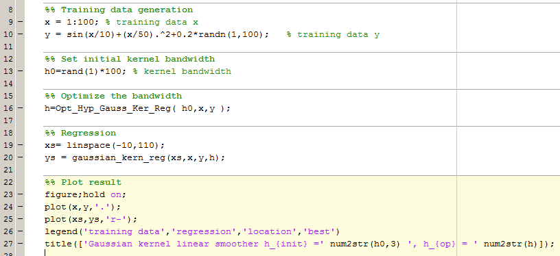
Gaussian Kernel Bandwidth Optimization with Matlab Code

In this article, I write on “Optimization of Gaussian Kernel Bandwidth” with Matlab Code.

First, I will briefly explain a methodology to optimize bandwidth values of Gaussian Kernel for regression problems. In other words, I will explain about “Cross validation Method.”

Then, I will share my Matlab code which optimizes the bandwidths of Gaussian Kernel for Gaussian Kernel Regression. For the theory and source code of the regression, read my previous posts <link for 1D input>, <link for multidimensional input>. This Matlab code can optimize bandwidths for multidimensional inputs. If you know the theory of cross validation, or if you don’t need to know the algorithm of my program, just download the zip file from the below link, then execute demo programs. Probably, you can use the program without big difficulties.

1. Bandwidth optimization by a cross validation method

The most common way to optimize a regression parameter is to use a cross validation method. If you want to know about the cross validation deeply, I want to recommend to read this article. Here I will shortly explain about the cross validation method that I am using. This is just a way of cross validation.

1. Randomly sample 75% of the data set, and put into the training data set, and put the remaining part into the test set.

2. Using the training data set, build a regression model. Based on the model, predict the outputs of the test set.

3. Compare between the predicted output, and the actual output. Then, find the best model (best bandwidth) to minimize the gap (e.g, RMSE) between the predicted and actual outputs.

2. Matlab code for the algorithm

You can download all functions and demo programs from the below link.

This program is for multidimensional inputs (of course, 1D is also OK). The most important function is Opt_Hyp_Gauss_Ker_Reg( h0,x,y ) and it requires Matlab optimization toolbox. I am attaching two demo programs and their results. I made these demo programs as much as I can. So, I believe that everybody can understand.

<Demo 1D>

<Demo 2D>

I wish this post can save your time and efforts in your work. If you have any question, please leave a reply.

-Mok-

—————————————————————————————————

I am Youngmok Yun, and writing about robotics theories and my research.

My main site is http://youngmok.com, and Korean ver. is http://yunyoungmok.tistory.com.

—————————————————————————————————

Gaussian Kernel Regression for Multidimensional Feature with Matlab code

4 Replies

Gaussian Kernel Regression for Multidimensional Feature with Matlab code (Gaussian Kernel or RBF Smoother)

I am sharing a Matlab code for Gaussian Kernel Regression algorithm for multidimensional input (feature).

In the previous post (link), I posted a theory of Gaussian Kernel Regression, and shared a Matlab code for one dimensional input. If you want to know about the theory, read the previous post. In the previous post, many visitors asked me for a multidimensional input version. Finally I made a Gaussian Kernel Regression Program for a general dimensional input

You can download the program from this link.

I wrote a demo program to show how to use the code as easy as possible.

The below is the demo program, and a demo result plot. In this demo program, the dimension of input is 2 because of visualization, but it is expendable to an arbitrary dimension.

For the optimization of kernel bandwidth, see my other article <Link>.

I wish this program can save your time and effort for your work.

If you have any question, please leave a reply.

—————————————————————————————————————————–

I am Youngmok Yun, and writing about robotics theories and my research.

My main site is http://youngmok.com, and Korean ver. is http://yunyoungmok.tistory.com.

—————————————————————————————————————————–

Gaussian kernel regression with Matlab code (Gaussian Kernel or RBF Smoother)

20 Replies

Gaussian kernel regression with Matlab code

In this article, I will explain Gaussian Kernel Regression (or Gaussian Kernel Smoother, or Gaussian Kernel-based linear regression, RBF kernel regression) algorithm. Plus I will share my Matlab code for this algorithm.

If you already know the theory. Just download from here. <Download>

You can see how to use this function from the below. It is super easy.

From here, I will explain the theory.

Basically, this algorithm is a kernel based linear smoother algorithm and just the kernel is the Gaussian kernel. With this smoothing method, we can find a nonlinear regression function.

The linear smoother is expressed with the below equation

$y^* = \frac{\sum^N_{i=1}K(x^*,x_i)y_i}{\sum^N_{i=1}K(x^*,x_i)}$

here x_i is the i_th training data input, y_i is the i_th training data output, K is a kernel function. x^* is a query point, y^* is the predicted output.

In this algorithm, we use the Gaussian Kernel which is expressed with the below equation. Another name of this functions is Radial Basis Function (RBF) because it is not exactly same with the Gaussian function.

$K(x^*,x_i)=\exp\left(-\frac{ (x^*-x_i)^2}{2b^2}\right)$

With these equation, we can smooth the training data outputs, thus we can find a regression function.

This program <Download> was made for one-dimensional inputs. If you need multi-dimension, ~~please leave a reply,~~ see this article. I recently made a new version for multidimensional input.

For the optimization of kernel bandwidth, see my other article <Link>.

Then good luck.

-Mok-

—————————————————————————————————————————–

I am Youngmok Yun, and writing about robotics theories and my research.

My main site is http://youngmok.com, and Korean ver. is http://yunyoungmok.tistory.com.

—————————————————————————————————————————–

Hill Type Muscle Model with Matlab Code

1 Reply

Hill Type Muscle Model with Matlab Code

In this post, I will write on the Hill type muscle model, and then, I will provide a Matlab code made for the model.

If you have a basic knowledge about the muscle tendon unit, and just want to download the Matlab code, just download from the following links

<Matlab m code> or <Matlab Simulink block>.

If you are familiar with Biomechanics, I think the best source to study a muscle tendon model is Zajac’s paper [4].

OK let’s go to the main writing.

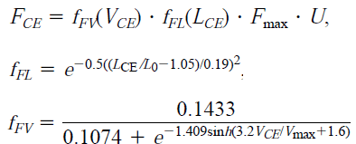
Generally, the muscle tendon unit is modeled by the below figure including a CE (controctile component element), PE (parallel elastic element), and SE (series elastic element). This is the Hill type muscle-tendon model. The CE and PE are elements for a muscle, and the SE is for a tendon. Sometimes the SE is ignored in modeling, depending on tendon type, because its stiffness is very high.

hill type muscle model [1]

The CE generates a contracting force on tendon, and the size of force is a function of the velocity/length of muscle as shown in the below equations. This is a general model, but sometimes the other model is used, depending on the type of muscle, if you want to know the detail refer [3].

Fce, Hill Type Muscle Model with Matlab Code

Force function of CE [2]

The PE element is modeled by the below equation. Again SE can be ignored, thus in my Matlab code, it is ignored.

Force of PE and SE, Hill Type Muscle Model with Matlab Code

Force of PE and SE [5]

Finally, we can make a model based on the above equations. In my code, I made a muscle-tendon model for finger muscles. If you want to model for the other muscle tendon unit, you have to search several parameters for the muscle.

You can download the Matlab code and Simulink code from below link. I made the same function with two different ways for user’s convenience.

<Matlab m code> or <Matlab Simulink block>.

[1]

E. M. Arnold, S. R. Ward, R. L. Lieber, and S. L. Delp, “A Model of the Lower Limb for Analysis of Human Movement,” Ann Biomed Eng, vol. 38, no. 2, pp. 269–279, Feb. 2010.

[2]

J. Rosen, M. B. Fuchs, and M. Arcan, “Performances of Hill-Type and Neural Network Muscle Models—Toward a Myosignal-Based Exoskeleton,” Computers and Biomedical Research, vol. 32, no. 5, pp. 415–439, Oct. 1999.

[3]

J. L. Sancho-Bru, A. Pérez-González, M. C. Mora, B. E. León, M. Vergara, J. L. Iserte, P. J. Rodríguez-Cervantes, and A. Morales, “Towards a realistic and self-contained biomechanical model of the hand,” 2011.

[4]

Z. Fe, “Muscle and tendon: properties, models, scaling, and application to biomechanics and motor control.,” Crit Rev Biomed Eng, vol. 17, no. 4, pp. 359–411, Dec. 1988.

[5]

P.-H. Kuo and A. D. Deshpande, “Contribution of passive properties of muscle-tendon units to the metacarpophalangeal joint torque of the index finger,” in Biomedical Robotics and Biomechatronics (BioRob), 2010 3rd IEEE RAS and EMBS International Conference on, 2010, pp. 288–294.

—————————————————————————————————————————–

I am Youngmok Yun, and writing about robotics theories and my research.

My main site is http://youngmok.com, and Korean ver. is http://yunyoungmok.tistory.com.

—————————————————————————————————————————–

Matlab compiler installation. If you have trouble after installation of Microsoft Windows SDK 7.1

1 Reply

Solution for the Matlab compiler installation. If you have trouble after installation of Microsoft Windows SDK 7.1

Today I am writing a tip to solve a Matlab compiler setup problem.

If you want to use MEX or any Matlab compiling technology, you need a compiler. Windows does not have a default compiler. So you have to install. If you don’t have any compiler, you would see the below message.

>> mex -setup

Welcome to mex -setup. This utility will help you set up
a default compiler. For a list of supported compilers, see
http://www.mathworks.com/support/compilers/R2013a/win64.html

Please choose your compiler for building MEX-files:

Would you like mex to locate installed compilers [y]/n? y

No supported SDK or compiler was found on this computer.
For a list of supported compilers, see
http://www.mathworks.com/support/compilers/R2013a/win64.html

Error using mex (line 206)
Unable to complete successfully.

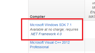
If you follow the link, you can install “Microsoft Windows SDK 7.1”

BUT, IMPORTANT, if you don’t have “.NET Framework 4.0,” you cannot install the compiler. As shown in the below figure, you MUST install .NET Framework 4.0 for installation of the windows compiler.

Matlab compiler problem, if you have trouble after the installation of Microsoft Windows SDK 7.1

Then, I wish this post can help to solve your problem.

Thank you.

—————————————————————————————————————————–

I am Youngmok Yun, and writing about robotics theories and my research.

My main site is http://youngmok.com, and Korean ver. is http://yunyoungmok.tistory.com.

—————————————————————————————————————————–

Parallel computation with Matlab, SPMD. Explanation with simple example code

2 Replies

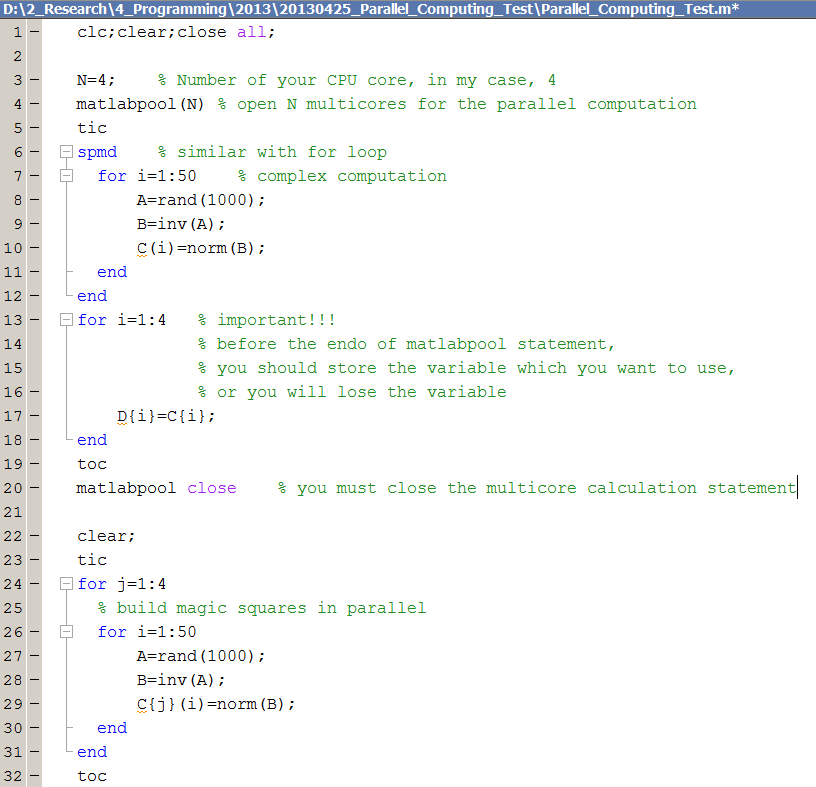
Today I’d like to introduce a parallel computation skill in Matlab.

I also heard that the use of parallel computation in Matlab is very easy. But it was better than my expectation. Wonderful!!

You need to know the usage of SPMD. It is pretty easy.

First let’s the code, you can also download this file in the attachment, click <here>.

The result is the below

Starting matlabpool using the ‘local’ configuration … connected to 4 labs.
Elapsed time is 120.482356 seconds.
Sending a stop signal to all the labs … stopped.
Elapsed time is 167.796932 seconds.

Because, I did many other works in the calculation time, Its result is not very fast, The slowest CPU core determined the final computation time. But its performance is really good if you have more than 4 multi cpu cores.

I wish this post can help your understanding about the use of SPMD in Matlab.

if you have any question, please leave me a comment below.

—————————————————————————————————

I am Youngmok Yun, and writing about robotics theories and my research.

My main site is http://youngmok.com, and Korean ver. is http://yunyoungmok.tistory.com.

—————————————————————————————————

Phase plane analysis and Matlab code toolbox

How to draw?

Given,

$\dot{x}_1=f_1(x_1,x_2)$

$\dot{x}_2=f_2(x_1,x_2)$

we can find the below equation

$\frac{dx_2}{dx_1}=\frac{f_2(x_1,x_2)}{f_1(x_1,x_2)}$

From $\frac{dx_2}{dx_1}$ , we can find the direction of the phase change at the point of $(x_1, x_2)$ .

Advantage:

It is an exact method. We can see the change of system’s state including transient response.
Simple graphical method. It is very intuitive and easy to understand its characteristics.

Limit:

Limited to the 2nd order system. It is expandable, but hard to visualize.

Reference

1. Lecture of Prof. Fernadez in Mech. Eng, The Univ. of Texas at Austin.

Matlab code for numerical hessian matrix

Example 1

Example 2

Share this:

Like this:

Share this:

Like this:

Lagrange Equation by MATLAB with Examples

1. Example system

2. Theoretical Background

3. Using Matlab symbolic toolbox

First, let’s define the symbols.

Second, find the position and velocities of the point masses.

Third, define the kinetic energy, and the potential energy.

Fourth, define the generalized forces, here torques.

Fifth, solve the Lagrangian equation

Sixth, rearrange the equations.

Seventh, substitute with y1,y2… variables.

Eighth, this is the result…. as you can see, it is almost impossible to solve by hand

4. Now it is ready!!! let’s run a simulation!

Share this:

Like this:

Gaussian Kernel Bandwidth Optimization with Matlab Code

1. Bandwidth optimization by a cross validation method

2. Matlab code for the algorithm

<Demo 1D>

<Demo 2D>

Share this:

Like this:

Gaussian Kernel Regression for Multidimensional Feature with Matlab code (Gaussian Kernel or RBF Smoother)

Share this:

Like this:

Gaussian kernel regression with Matlab code

Share this:

Like this:

Hill Type Muscle Model with Matlab Code

Share this:

Like this:

Solution for the Matlab compiler installation. If you have trouble after installation of Microsoft Windows SDK 7.1

Share this:

Like this:

Share this:

Like this:

How to draw?

Advantage:

Limit:

Reference

Share this:

Like this: