
Lagrange Equation by MATLAB with Examples
In this post, I will explain how to derive a dynamic equation with Lagrange Equation by MATLAB with Examples. As an example, I will derive a dynamic model of a three-DOF arm manipulator (or triple pendulum). Of course you may get a dynamic model for a two-DOF arm manipulator by simply removing several lines. I am attaching demo codes for both two and three DOF arm manipulators.
If you know all theories and necessary skills and if you just want source code, you can just download from here.
In the attached file, “Symb_Development_3DOF.m” generates a dynamic model. “main_sim_three_dof_arm.m” runs a simulation. You may get a result like this.
1. Example system
Let’s suppose a three DOF arm manipulator shown in the below figure. I am assuming all of masses (M1, M2, M3) exist at the end of links for simplicity. Three actuators exist at each joint, and directly actuate the torques (u1,u2,u3). The manipulator kinematics is governed by three joint angles (q1, q2, q3).
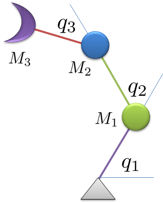
three DOF arm manipulator
2. Theoretical Background
We will get a dynamic equation of this system by using Lagrangian mechanics. If you do not have a background knowledge of Lagrangian mechanics, please refer here.
The general dynamic equation is obtained by
Where, T is the total kinetic energy, V is the total potential energy of the system. where is the generalized force, t is time,
is the generalized coordinates,
is the generalized velocity. For the example of three-DOF arm manipulator problem,
is the torque at the j-th joint,
is the angle of the j-th joint,
is the angular velocity of the j-th joint.
3. Using Matlab symbolic toolbox
First, let’s define the symbols.
I am using x to represent q, xd for , xdd for
L is the length of each link. u is the torque of each joint. g is the gravity constant.
syms M1 M2 M3;
syms x1 x1d x1dd x2 x2d x2dd x3 x3d x3dd;
syms L1 L2 L3;
syms u1 u2 u3;
syms g
Second, find the position and velocities of the point masses.
p1x = L1cos(x1);
p1y = L1sin(x1);
p2x = p1x+L2cos(x1+x2);
p2y = p1y+L2sin(x1+x2);
p3x = p2x+L3cos(x1+x2+x3);
p3y = p2y+L3sin(x1+x2+x3);
v1x = -L1sin(x1)x1d;
v1y = +L1cos(x1)x1d;
v2x = v1x-L2sin(x1+x2)(x1d+x2d);
v2y = v1y+L2cos(x1+x2)(x1d+x2d);
v3x = v2x – L3sin(x1+x2+x3)(x1d+x2d+x3d);
v3y = v2y + L3cos(x1+x2+x3)(x1d+x2d+x3d);
Third, define the kinetic energy, and the potential energy.
KE = 0.5M1( v1x^2 + v1y^2) + 0.5M2( v2x^2 + v2y^2) + 0.5M3( v3x^2 + v3y^2);
KE = simplify(KE);
PE = M1gp1y + M2gp2y + M3gp3y;
PE = simplify(PE);
Fourth, define the generalized forces, here torques.
Px1 = u1;
Px2 = u2;
Px3 = u3;
Fifth, solve the Lagrangian equation
We have to get the Lagrangian eqn.
Let’s obtain step by step.
is obtained by
pKEpx1d = diff(KE,x1d);
To calculate, , we need the chain rule, that is
ddtpKEpx1d = diff(pKEpx1d,x1)x1d+ …
diff(pKEpx1d,x1d)x1dd+ …
diff(pKEpx1d,x2)x2d + …
diff(pKEpx1d,x2d)x2dd + …
diff(pKEpx1d,x3)x3d + …
diff(pKEpx1d,x3d)x3dd;
are easily obtained by
pKEpx1 = diff(KE,x1);
pPEpx1 = diff(PE,x1);
By summing all equations,
eqx1 = simplify( ddtpKEpx1d – pKEpx1 + pPEpx1 – Px1);
By repeating these procedures, we can get all governing equations.
Sixth, rearrange the equations.
We love more simplified forms like
For this form, we need to rearrange the equations by
Sol = solve(eqx1,eqx2,eqx3,’x1dd,x2dd,x3dd’);
Sol.x1dd = simplify(Sol.x1dd);
Sol.x2dd = simplify(Sol.x2dd);
Sol.x3dd = simplify(Sol.x3dd);
Seventh, substitute with y1,y2… variables.
Just for easier implementation of symbolic codes, let’s substitute x1, x1d, x2, … with y1,y2….
syms y1 y2 y3 y4 y5 y6
fx1=subs(Sol.x1dd,{x1,x1d,x2,x2d,x3,x3d},{y1,y2,y3,y4,y5,y6})
fx2=subs(Sol.x2dd,{x1,x1d,x2,x2d,x3,x3d},{y1,y2,y3,y4,y5,y6})
fx3=subs(Sol.x3dd,{x1,x1d,x2,x2d,x3,x3d},{y1,y2,y3,y4,y5,y6})
Eighth, this is the result…. as you can see, it is almost impossible to solve by hand
fx1 =
(L2L3M2u1 – L2L3M2u2 + L2L3M3u1 – L2L3M3u2 – L1L3M2u2cos(y3) + L1L3M2u3cos(y3) – L1L3M3u2cos(y3) + L1L3M3u3cos(y3) – L2L3M3u1cos(y5)^2 + L2L3M3u2cos(y5)^2 + L1L2^2L3M2^2y2^2sin(y3) + L1L2^2L3M2^2y4^2sin(y3) – L1L2L3M2^2gcos(y1) + (L1^2L2L3M2^2y2^2sin(2y3))/2 + L1L2M2u3sin(y3)sin(y5) + L1L2M3u3sin(y3)sin(y5) + L1L3M3u2cos(y3)cos(y5)^2 – L1L3M3u3cos(y3)cos(y5)^2 + L1L2^2L3M2M3y2^2sin(y3) + L1L2^2L3M2M3y4^2sin(y3) – L1L2L3M1M2gcos(y1) – L1L2L3M1M3gcos(y1) – L1L2L3M2M3gcos(y1) + 2L1L2^2L3M2^2y2y4sin(y3) + (L1^2L2L3M2M3y2^2sin(2y3))/2 – L1L3M3u2cos(y5)sin(y3)sin(y5) + L1L3M3u3cos(y5)sin(y3)sin(y5) + L1L2L3M2^2gcos(y1)cos(y3)^2 – L1L2L3M2^2gcos(y3)sin(y1)sin(y3) + 2L1L2^2L3M2M3y2y4sin(y3) + L1L2L3M2M3gcos(y1)cos(y3)^2 + L1L2L3M1M3gcos(y1)cos(y5)^2 + L1L2L3^2M2M3y2^2cos(y5)sin(y3) + L1L2L3^2M2M3y4^2cos(y5)sin(y3) + L1L2L3^2M2M3y6^2cos(y5)sin(y3) + 2L1L2L3^2M2M3y2y4cos(y5)sin(y3) + 2L1L2L3^2M2M3y2y6cos(y5)sin(y3) + 2L1L2L3^2M2M3y4y6cos(y5)sin(y3) – L1L2L3M2M3gcos(y3)sin(y1)sin(y3))/(L1^2L2L3(M2^2 – M2^2cos(y3)^2 + M1M2 + M1M3 + M2M3 – M2M3cos(y3)^2 – M1M3*cos(y5)^2))
fx2 =
-(2L1^2L3M1u3 – 2L1^2L3M1u2 – 2L1^2L3M2u2 + 2L2^2L3M2u1 + 2L1^2L3M2u3 – L1^2L3M3u2 – 2L2^2L3M2u2 + L2^2L3M3u1 + L1^2L3M3u3 – L2^2L3M3u2 + L1L2^2M2u3cos(y3 – y5) + L1L2^2M3u3cos(y3 – y5) – L1^2L2M2u3cos(2y3 + y5) – L1^2L2M3u3cos(2y3 + y5) – L2^2L3M3u1cos(2y5) + L2^2L3M3u2cos(2y5) + L1^2L3M3u2cos(2y3 + 2y5) – L1^2L3M3u3cos(2y3 + 2y5) – L1L2^2M2u3cos(y3 + y5) – L1L2^2M3u3cos(y3 + y5) + 2L1^2L2M1u3cos(y5) + L1^2L2M2u3cos(y5) + L1^2L2M3u3cos(y5) + 2L1L2^3L3M2^2y2^2sin(y3) + 2L1^3L2L3M2^2y2^2sin(y3) + 2L1L2^3L3M2^2y4^2sin(y3) – L1L2L3M3u1cos(y3 + 2y5) + 2L1L2L3M3u2cos(y3 + 2y5) – L1L2L3M3u3cos(y3 + 2y5) + L1^2L2L3M2^2gcos(y1 + y3) – L1L2^2L3M2^2gcos(y1) – L1^2L2L3M2^2gcos(y1 – y3) + L1L2^2L3M2^2gcos(y1 + 2y3) + 2L1^2L2^2L3M2^2y2^2sin(2y3) + L1^2L2^2L3M2^2y4^2sin(2y3) + 2L1L2L3M2u1cos(y3) – 4L1L2L3M2u2cos(y3) + L1L2L3M3u1cos(y3) + 2L1L2L3M2u3cos(y3) – 2L1L2L3M3u2cos(y3) + L1L2L3M3u3cos(y3) + 2L1^3L2L3M1M2y2^2sin(y3) + L1^3L2L3M1M3y2^2sin(y3) + 2L1L2^3L3M2M3y2^2sin(y3) + 2L1^3L2L3M2M3y2^2sin(y3) + 2L1L2^3L3M2M3y4^2sin(y3) + 4L1L2^3L3M2^2y2y4sin(y3) – (L1^2L2L3M1M3gcos(y1 + y3 + 2y5))/2 – L1^3L2L3M1M3y2^2sin(y3 + 2y5) + L1L2^2L3^2M2M3y2^2sin(y3 + y5) + L1L2^2L3^2M2M3y4^2sin(y3 + y5) + L1L2^2L3^2M2M3y6^2sin(y3 + y5) + L1^2L2L3M1M2gcos(y1 + y3) + (L1^2L2L3M1M3gcos(y1 + y3))/2 + L1^2L2L3M2M3gcos(y1 + y3) – 2L1^2L2L3^2M1M3y2^2sin(y5) – L1^2L2L3^2M2M3y2^2sin(y5) – 2L1^2L2L3^2M1M3y4^2sin(y5) – L1^2L2L3^2M2M3y4^2sin(y5) – 2L1^2L2L3^2M1M3y6^2sin(y5) – L1^2L2L3^2M2M3y6^2sin(y5) – 2L1L2^2L3M1M2gcos(y1) – L1L2^2L3M1M3gcos(y1) – L1L2^2L3M2M3gcos(y1) + (L1^2L2L3M1M3gcos(y1 – y3 – 2y5))/2 + L1L2^2L3^2M2M3y2^2sin(y3 – y5) + L1^2L2L3^2M2M3y2^2sin(2y3 + y5) + L1L2^2L3^2M2M3y4^2sin(y3 – y5) + L1^2L2L3^2M2M3y4^2sin(2y3 + y5) + L1L2^2L3^2M2M3y6^2sin(y3 – y5) + L1^2L2L3^2M2M3y6^2sin(2y3 + y5) – L1^2L2L3M1M2gcos(y1 – y3) – (L1^2L2L3M1M3gcos(y1 – y3))/2 – L1^2L2L3M2M3gcos(y1 – y3) + L1L2^2L3M2M3gcos(y1 + 2y3) + (L1L2^2L3M1M3gcos(y1 – 2y5))/2 + (L1L2^2L3M1M3gcos(y1 + 2y5))/2 + 2L1^2L2^2L3M2M3y2^2sin(2y3) – L1^2L2^2L3M1M3y2^2sin(2y5) + L1^2L2^2L3M2M3y4^2sin(2y3) – L1^2L2^2L3M1M3y4^2sin(2y5) + 2L1^2L2^2L3M2^2y2y4sin(2y3) + 4L1L2^3L3M2M3y2y4sin(y3) + 2L1L2^2L3^2M2M3y2y4sin(y3 + y5) + 2L1L2^2L3^2M2M3y2y6sin(y3 + y5) + 2L1L2^2L3^2M2M3y4y6sin(y3 + y5) – 4L1^2L2L3^2M1M3y2y4sin(y5) – 2L1^2L2L3^2M2M3y2y4sin(y5) – 4L1^2L2L3^2M1M3y2y6sin(y5) – 2L1^2L2L3^2M2M3y2y6sin(y5) – 4L1^2L2L3^2M1M3y4y6sin(y5) – 2L1^2L2L3^2M2M3y4y6sin(y5) + 2L1L2^2L3^2M2M3y2y4sin(y3 – y5) + 2L1^2L2L3^2M2M3y2y4sin(2y3 + y5) + 2L1L2^2L3^2M2M3y2y6sin(y3 – y5) + 2L1^2L2L3^2M2M3y2y6sin(2y3 + y5) + 2L1L2^2L3^2M2M3y4y6sin(y3 – y5) + 2L1^2L2L3^2M2M3y4y6sin(2y3 + y5) + 2L1^2L2^2L3M2M3y2y4sin(2y3) – 2L1^2L2^2L3M1M3y2y4sin(2y5))/(L1^2L2^2L3(M2^2 – M2^2cos(2y3) + 2M1M2 + M1M3 + M2M3 – M2M3cos(2y3) – M1M3cos(2*y5)))
fx3 =
-(L1L3^2M3^2u2 – L1L2^2M3^2u3 – L1L2^2M2^2u3 – L1L3^2M3^2u3 – L2L3^2M3^2u1cos(y3) + L2L3^2M3^2u2cos(y3) – 2L1L2^2M1M2u3 – 2L1L2^2M1M3u3 + 2L1L3^2M1M3u2 – 2L1L2^2M2M3u3 – 2L1L3^2M1M3u3 + 2L1L3^2M2M3u2 – 2L1L3^2M2M3u3 + L1L2^2M2^2u3cos(2y3) + L1L2^2M3^2u3cos(2y3) + L1L3^2M3^2u2sin(2y3)sin(2y5) – L1L3^2M3^2u3sin(2y3)sin(2y5) + L1L2L3M3^2u2cos(y5) – 2L1L2L3M3^2u3cos(y5) – 2L2L3^2M2M3u1cos(y3) + 2L2L3^2M2M3u2cos(y3) – 2L2^2L3M3^2u1sin(y3)sin(y5) + 2L2^2L3M3^2u2sin(y3)sin(y5) + L2L3^2M3^2u1cos(2y5)cos(y3) – L2L3^2M3^2u2cos(2y5)cos(y3) + 2L1L2^2M2M3u3cos(2y3) – L2L3^2M3^2u1sin(2y5)sin(y3) + L2L3^2M3^2u2sin(2y5)sin(y3) – L1L3^2M3^2u2cos(2y3)cos(2y5) + L1L3^2M3^2u3cos(2y3)cos(2y5) – L1L2^2L3^2M2M3^2y2^2sin(2y3) – L1L2^2L3^2M2^2M3y2^2sin(2y3) + 2L1L2^2L3^2M1M3^2y2^2sin(2y5) – L1L2^2L3^2M2M3^2y4^2sin(2y3) – L1L2^2L3^2M2^2M3y4^2sin(2y3) + 2L1L2^2L3^2M1M3^2y4^2sin(2y5) + L1L2^2L3^2M1M3^2y6^2sin(2y5) + 2L1L2L3M1M3u2cos(y5) – 4L1L2L3M1M3u3cos(y5) + L1L2L3M2M3u2cos(y5) – 2L1L2L3M2M3u3cos(y5) – 2L2^2L3M2M3u1sin(y3)sin(y5) + 2L2^2L3M2M3u2sin(y3)sin(y5) + 2L1L2L3^3M1M3^2y2^2sin(y5) + 2L1L2^3L3M1M3^2y2^2sin(y5) + L1L2L3^3M2M3^2y2^2sin(y5) + 2L1L2L3^3M1M3^2y4^2sin(y5) + 2L1L2^3L3M1M3^2y4^2sin(y5) + L1L2L3^3M2M3^2y4^2sin(y5) + 2L1L2L3^3M1M3^2y6^2sin(y5) + L1L2L3^3M2M3^2y6^2sin(y5) – L1L2L3M3^2u2cos(2y3)cos(y5) + 2L1L2L3M3^2u3cos(2y3)cos(y5) + L1L2L3M3^2u2sin(2y3)sin(y5) – 2L1L2L3M3^2u3sin(2y3)sin(y5) – L1^2L2L3^2M1M3^2y2^2sin(y3) – 2L1^2L2L3^2M2M3^2y2^2sin(y3) – 2L1^2L2L3^2M2^2M3y2^2sin(y3) – 2L1L2^2L3^2M2M3^2y2y4sin(2y3) – 2L1L2^2L3^2M2^2M3y2y4sin(2y3) + 4L1L2^2L3^2M1M3^2y2y4sin(2y5) + 2L1L2^2L3^2M1M3^2y2y6sin(2y5) + 2L1L2^2L3^2M1M3^2y4y6sin(2y5) + 2L1L2^3L3M1M2M3y2^2sin(y5) + 2L1L2^3L3M1M2M3y4^2sin(y5) – L1L2L3M2M3u2cos(2y3)cos(y5) + 2L1L2L3M2M3u3cos(2y3)cos(y5) + 4L1L2L3^3M1M3^2y2y4sin(y5) + 4L1L2^3L3M1M3^2y2y4sin(y5) + 2L1L2L3^3M2M3^2y2y4sin(y5) + 4L1L2L3^3M1M3^2y2y6sin(y5) + 2L1L2L3^3M2M3^2y2y6sin(y5) + 4L1L2L3^3M1M3^2y4y6sin(y5) + 2L1L2L3^3M2M3^2y4y6sin(y5) + L1L2L3M2M3u2sin(2y3)sin(y5) – 2L1L2L3M2M3u3sin(2y3)sin(y5) – L1L2L3^3M2M3^2y2^2cos(2y3)sin(y5) – L1L2L3^3M2M3^2y2^2sin(2y3)cos(y5) – L1L2L3^3M2M3^2y4^2cos(2y3)sin(y5) – L1L2L3^3M2M3^2y4^2sin(2y3)cos(y5) – L1L2L3^3M2M3^2y6^2cos(2y3)sin(y5) – L1L2L3^3M2M3^2y6^2sin(2y3)cos(y5) + 2L1^2L2^2L3M1M3^2y2^2cos(y3)sin(y5) – 2L1^2L2L3^2M1M2M3y2^2sin(y3) + L1L2L3^2M1M3^2gsin(y1)sin(y3) + 2L1L2L3^2M2M3^2gsin(y1)sin(y3) + 2L1L2L3^2M2^2M3gsin(y1)sin(y3) + L1^2L2L3^2M1M3^2y2^2cos(2y5)sin(y3) + L1^2L2L3^2M1M3^2y2^2sin(2y5)cos(y3) – L1L2L3^2M1M3^2gcos(2y5)sin(y1)sin(y3) – L1L2L3^2M1M3^2gsin(2y5)cos(y3)sin(y1) + 4L1L2^3L3M1M2M3y2y4sin(y5) + 2L1^2L2^2L3M1M2M3y2^2cos(y3)sin(y5) – 2L1L2L3^3M2M3^2y2y4cos(2y3)sin(y5) – 2L1L2L3^3M2M3^2y2y4sin(2y3)cos(y5) – 2L1L2L3^3M2M3^2y2y6cos(2y3)sin(y5) – 2L1L2L3^3M2M3^2y2y6sin(2y3)cos(y5) – 2L1L2L3^3M2M3^2y4y6cos(2y3)sin(y5) – 2L1L2L3^3M2M3^2y4y6sin(2y3)cos(y5) – 2L1L2^2L3M1M3^2gcos(y3)sin(y1)sin(y5) + 2L1L2L3^2M1M2M3gsin(y1)sin(y3) – 2L1L2^2L3M1M2M3gcos(y3)sin(y1)sin(y5))/(L1L2^2L3^2M3(M2^2 – M2^2cos(2y3) + 2M1M2 + M1M3 + M2M3 – M2M3cos(2y3) – M1M3cos(2y5)))
4. Now it is ready!!! let’s run a simulation!
copy the result and paste the symbols in a Matlab function. Then, run an ODE with the function.
A sample code is here.
In the attached file, “Symb_Development_3DOF.m” generates a dynamic model. “main_sim_three_dof_arm.m” runs a simulation. Then, you can get this result.
So far, I have explained how to derive a Lagrange Equation by MATLAB with Examples. I hope that this post helps your project and save your time. Please leave a message if you have any question.
Update on 02/21/2016
I updated some code and posting about typo. “simple” -> “simplify” There is no function “simple” Now all programs are running well.
-Mok-
Reference
[1] http://en.wikipedia.org/wiki/Lagrangian_mechanics
[3] http://www.mathworks.com/matlabcentral/fileexchange/23037-lagrange-s-equations


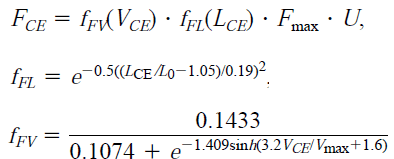
![hill type muscle model [1], Hill Type Muscle Model with Matlab Code](https://i0.wp.com/youngmok.com/wp-content/uploads/2013/11/hill_type_muscle_model.png)