Category Archives: Programming

Site to learn TCP/IP programming in Linux

ADS7813 ADS7812 Arduino Code

1. ADS7813 ADS7812: Low-Power, Serial 16/12-Bit Sampling ANALOG-TO-DIGITAL CONVERTER

ADS7813/ADS7812 is a general purpose ADC made by Texas Instrument, and it is pretty easy to operate through SPI. You can see the datasheet from here.

2. Connections

This is the electric connection diagram that I used for my setup. I have used ADS7813 but all configurations are same with ADS7812. Just only difference is that the resolution of ADS7812 is 12bit .

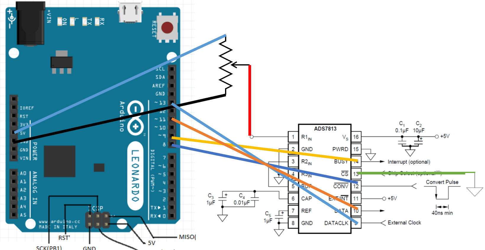
This electric connection is actually a reference connection provided by TI datasheet. With this connection, I made the Arduino code like this.

3. Arduino code

#include <SPI.h>

const int i_conv = 8;
const int i_busy = 9;

void setup() {
  Serial.begin(9600);

  // start the SPI library:
  SPI.begin();

  pinMode(i_conv, OUTPUT);
  pinMode(i_busy, INPUT);

  delay(100);
}

void loop(){

  bool i_busy_status=1;
  byte data1;
  byte data2;
  digitalWrite(i_conv,HIGH);
  delay(1);
  digitalWrite(i_conv,LOW);
  while ( digitalRead(i_busy) == LOW ){
  }
  data1 = SPI.transfer(0x00);
  data2 = SPI.transfer(0x00);
  digitalWrite(i_conv,HIGH);
  Serial.print(data1);
  Serial.print(" ");
  Serial.print(data2);
  Serial.print("\n");
 
}

I included only very essential part so that you might be easily able to understand the code. I am also attaching the code. <Download>

4. Operation video

This is the video showing the operation.

Nowadays I am playing with an Arduino, and I got many helps from communities. I hope this ADS7813 ADS7812 Arduino Code can help your project.

Matlab Code for Numerical Hessian Matrix

2 Replies

Matlab code for numerical hessian matrix

In this post, I am sharing a Malab code calculating a numerical hessian matrix.

You can download here.

You can use NumHessian.m with this syntax.

function hf = NumHessian(f,x0,varargin)

You can understand how to use simply by reading these two simple examples.

Example 1

>> NumHessian(@cos,0)

ans =

-1.0000

Example 2

function y=test_func(x,a)
y=ax(1)x(2)*x(3);

>> NumHessian(@test_func,[1 2 3]’,2)

ans =

0 6.0000 4.0000
5.9999 -0.0001 1.9998
3.9999 2.0000 0

I hope this Matlab code for numerical Hessian matrix helps your projects

This Matlab code is based on another Matlab function, NumJacob, which calculates a numerical Jacobian matrix. If you are interested in this, visit here.

If you want to know the theory on Hessian matrix, please read this Wiki.

I acknowledge that this code is originally made by Parviz Khavari, a visitor of this blog, and I modified to post here.

Compiling a Matlab C code with GCC/G++

6 Replies

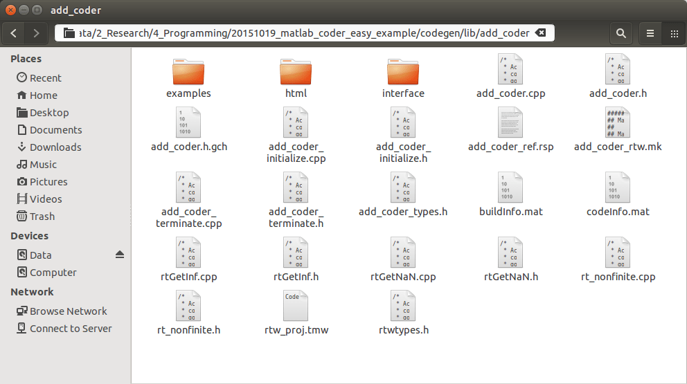
In this post, I am sharing how to compile a C code generated by Matlab C coder with GCC compiler. Let me explain with an example.

1. Generating a C code with Matlab C coder.

I will use a very simple Matlab code, and the below is the code

function y = add_coder(a,b)
y=a+b

With the Matlab C coder, let’s auto-generate the C code. You have to specify the types of variables and some other options. If you just read the dialog box, it might not be difficult.

As a result, you can see this kind of result. If your Matlab version is not 2015, it might be little different, but its big flow is almost same.

2. Let’s compile the code generated by Matlab C coder

This is my main.cpp file that is modified from the auto-generated main.cpp by Matlab C coder

#include "rt_nonfinite.h"
#include "add_coder.h"
#include "add_coder_terminate.h"
#include "add_coder_initialize.h"
#include "stdio.h"

int main()
{
  /* Initialize the application.
     You do not need to do this more than one time. */
  add_coder_initialize();

  /* Invoke the entry-point functions.
     You can call entry-point functions multiple times. */
  double a=10;
  double b=20.0;
  double y;
  y = add_coder(a, b);
  printf("y: %lf\n",y);

  /* Terminate the application.
     You do not need to do this more than one time. */
  add_coder_terminate();
  return 0;
}

I located this main.cpp file with other all codes.

Now let’s compile all codes. Just compile main.cpp with all other cpp files. like this.

I am attaching all related files as a zip file. <Download>

Isn’t it easy??!!!

Have a good day~~!

Vertex angle from three points, Matlab code

Lagrange Equation by MATLAB with Examples

12 Replies

Lagrange Equation by MATLAB with Examples

In this post, I will explain how to derive a dynamic equation with Lagrange Equation by MATLAB with Examples. As an example, I will derive a dynamic model of a three-DOF arm manipulator (or triple pendulum). Of course you may get a dynamic model for a two-DOF arm manipulator by simply removing several lines. I am attaching demo codes for both two and three DOF arm manipulators.

If you know all theories and necessary skills and if you just want source code, you can just download from here.

<Download>

In the attached file, “Symb_Development_3DOF.m” generates a dynamic model. “main_sim_three_dof_arm.m” runs a simulation. You may get a result like this.

1. Example system

Let’s suppose a three DOF arm manipulator shown in the below figure. I am assuming all of masses (M1, M2, M3) exist at the end of links for simplicity. Three actuators exist at each joint, and directly actuate the torques (u1,u2,u3). The manipulator kinematics is governed by three joint angles (q1, q2, q3).

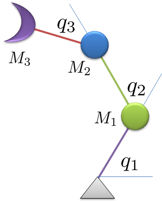
three DOF arm manipulator

2. Theoretical Background

We will get a dynamic equation of this system by using Lagrangian mechanics. If you do not have a background knowledge of Lagrangian mechanics, please refer here.

The general dynamic equation is obtained by

$\frac{d}{dt}\left( \frac{\partial T}{\partial \dot{q}_j}\right ) - \frac{\partial T}{\partial q_j} + \frac{\partial V}{\partial q_j} = P_j$

Where, T is the total kinetic energy, V is the total potential energy of the system. where $P_j$ is the generalized force, t is time, $q_j$ is the generalized coordinates, $\dot{q}_j$ is the generalized velocity. For the example of three-DOF arm manipulator problem, $P_j$ is the torque at the j-th joint, $q_j$ is the angle of the j-th joint, $\dot{q}_j$ is the angular velocity of the j-th joint.

3. Using Matlab symbolic toolbox

First, let’s define the symbols.

I am using x to represent q, xd for $\dot{q}$ , xdd for $\ddot{q}$ L is the length of each link. u is the torque of each joint. g is the gravity constant.

syms M1 M2 M3;
syms x1 x1d x1dd x2 x2d x2dd x3 x3d x3dd;
syms L1 L2 L3;
syms u1 u2 u3;
syms g

Second, find the position and velocities of the point masses.

p1x = L1cos(x1);
p1y = L1sin(x1);
p2x = p1x+L2cos(x1+x2);
p2y = p1y+L2sin(x1+x2);
p3x = p2x+L3cos(x1+x2+x3);
p3y = p2y+L3sin(x1+x2+x3);

v1x = -L1sin(x1)x1d;
v1y = +L1cos(x1)x1d;
v2x = v1x-L2sin(x1+x2)(x1d+x2d);
v2y = v1y+L2cos(x1+x2)(x1d+x2d);
v3x = v2x – L3sin(x1+x2+x3)(x1d+x2d+x3d);
v3y = v2y + L3cos(x1+x2+x3)(x1d+x2d+x3d);

Third, define the kinetic energy, and the potential energy.

KE = 0.5M1( v1x^2 + v1y^2) + 0.5M2( v2x^2 + v2y^2) + 0.5M3( v3x^2 + v3y^2);
KE = simplify(KE);

PE = M1gp1y + M2gp2y + M3gp3y;
PE = simplify(PE);

Fourth, define the generalized forces, here torques.

Px1 = u1;
Px2 = u2;
Px3 = u3;

Fifth, solve the Lagrangian equation

We have to get the Lagrangian eqn. $\frac{d}{dt}\left( \frac{\partial T}{\partial \dot{q}_j}\right ) - \frac{\partial T}{\partial q_j} + \frac{\partial V}{\partial q_j} = P_j$

Let’s obtain step by step.

$\left( \frac{\partial T}{\partial \dot{q}}\right )$ is obtained by

pKEpx1d = diff(KE,x1d);

To calculate, $\frac{d}{dt}\left( \frac{\partial T}{\partial \dot{q}}\right )$ , we need the chain rule, that is $\frac{d}{dt}\left( \frac{\partial T}{\partial \dot{q}_j}\right )= \sum^{3}_i \left\{ \frac{\partial }{\partial {q}_i}\left( \frac{\partial T}{\partial \dot{q}_j}\right )\frac{dq_i}{dt} + \frac{\partial }{\partial \dot{q}_i}\left( \frac{\partial T}{\partial {q}_j}\right )\frac{d \dot{q}_i}{dt} \right\}$

ddtpKEpx1d = diff(pKEpx1d,x1)x1d+ …
diff(pKEpx1d,x1d)x1dd+ …
diff(pKEpx1d,x2)x2d + …
diff(pKEpx1d,x2d)x2dd + …
diff(pKEpx1d,x3)x3d + …
diff(pKEpx1d,x3d)x3dd;

$\frac{\partial T}{\partial q_j}, \frac{\partial V}{\partial q_j}$ are easily obtained by

pKEpx1 = diff(KE,x1);
pPEpx1 = diff(PE,x1);

By summing all equations,

eqx1 = simplify( ddtpKEpx1d – pKEpx1 + pPEpx1 – Px1);

By repeating these procedures, we can get all governing equations.

Sixth, rearrange the equations.

We love more simplified forms like

$\frac{d}{dt} \begin{bmatrix} x_1\\ \dot{x}_1\\ x_2\\ \dot{x}_2\\ x_3\\ \dot{x}_3 \end{bmatrix}= f(x_1,\dot{x}_1,x_2,\dot{x}_2,x_3,\dot{x}_3)$

For this form, we need to rearrange the equations by

Sol = solve(eqx1,eqx2,eqx3,’x1dd,x2dd,x3dd’);
Sol.x1dd = simplify(Sol.x1dd);
Sol.x2dd = simplify(Sol.x2dd);
Sol.x3dd = simplify(Sol.x3dd);

Seventh, substitute with y1,y2… variables.

Just for easier implementation of symbolic codes, let’s substitute x1, x1d, x2, … with y1,y2….

syms y1 y2 y3 y4 y5 y6
fx1=subs(Sol.x1dd,{x1,x1d,x2,x2d,x3,x3d},{y1,y2,y3,y4,y5,y6})
fx2=subs(Sol.x2dd,{x1,x1d,x2,x2d,x3,x3d},{y1,y2,y3,y4,y5,y6})
fx3=subs(Sol.x3dd,{x1,x1d,x2,x2d,x3,x3d},{y1,y2,y3,y4,y5,y6})

Eighth, this is the result…. as you can see, it is almost impossible to solve by hand

fx1 =

(L2L3M2u1 – L2L3M2u2 + L2L3M3u1 – L2L3M3u2 – L1L3M2u2cos(y3) + L1L3M2u3cos(y3) – L1L3M3u2cos(y3) + L1L3M3u3cos(y3) – L2L3M3u1cos(y5)^2 + L2L3M3u2cos(y5)^2 + L1L2^2L3M2^2y2^2sin(y3) + L1L2^2L3M2^2y4^2sin(y3) – L1L2L3M2^2gcos(y1) + (L1^2L2L3M2^2y2^2sin(2y3))/2 + L1L2M2u3sin(y3)sin(y5) + L1L2M3u3sin(y3)sin(y5) + L1L3M3u2cos(y3)cos(y5)^2 – L1L3M3u3cos(y3)cos(y5)^2 + L1L2^2L3M2M3y2^2sin(y3) + L1L2^2L3M2M3y4^2sin(y3) – L1L2L3M1M2gcos(y1) – L1L2L3M1M3gcos(y1) – L1L2L3M2M3gcos(y1) + 2L1L2^2L3M2^2y2y4sin(y3) + (L1^2L2L3M2M3y2^2sin(2y3))/2 – L1L3M3u2cos(y5)sin(y3)sin(y5) + L1L3M3u3cos(y5)sin(y3)sin(y5) + L1L2L3M2^2gcos(y1)cos(y3)^2 – L1L2L3M2^2gcos(y3)sin(y1)sin(y3) + 2L1L2^2L3M2M3y2y4sin(y3) + L1L2L3M2M3gcos(y1)cos(y3)^2 + L1L2L3M1M3gcos(y1)cos(y5)^2 + L1L2L3^2M2M3y2^2cos(y5)sin(y3) + L1L2L3^2M2M3y4^2cos(y5)sin(y3) + L1L2L3^2M2M3y6^2cos(y5)sin(y3) + 2L1L2L3^2M2M3y2y4cos(y5)sin(y3) + 2L1L2L3^2M2M3y2y6cos(y5)sin(y3) + 2L1L2L3^2M2M3y4y6cos(y5)sin(y3) – L1L2L3M2M3gcos(y3)sin(y1)sin(y3))/(L1^2L2L3(M2^2 – M2^2cos(y3)^2 + M1M2 + M1M3 + M2M3 – M2M3cos(y3)^2 – M1M3*cos(y5)^2))

fx2 =

-(2L1^2L3M1u3 – 2L1^2L3M1u2 – 2L1^2L3M2u2 + 2L2^2L3M2u1 + 2L1^2L3M2u3 – L1^2L3M3u2 – 2L2^2L3M2u2 + L2^2L3M3u1 + L1^2L3M3u3 – L2^2L3M3u2 + L1L2^2M2u3cos(y3 – y5) + L1L2^2M3u3cos(y3 – y5) – L1^2L2M2u3cos(2y3 + y5) – L1^2L2M3u3cos(2y3 + y5) – L2^2L3M3u1cos(2y5) + L2^2L3M3u2cos(2y5) + L1^2L3M3u2cos(2y3 + 2y5) – L1^2L3M3u3cos(2y3 + 2y5) – L1L2^2M2u3cos(y3 + y5) – L1L2^2M3u3cos(y3 + y5) + 2L1^2L2M1u3cos(y5) + L1^2L2M2u3cos(y5) + L1^2L2M3u3cos(y5) + 2L1L2^3L3M2^2y2^2sin(y3) + 2L1^3L2L3M2^2y2^2sin(y3) + 2L1L2^3L3M2^2y4^2sin(y3) – L1L2L3M3u1cos(y3 + 2y5) + 2L1L2L3M3u2cos(y3 + 2y5) – L1L2L3M3u3cos(y3 + 2y5) + L1^2L2L3M2^2gcos(y1 + y3) – L1L2^2L3M2^2gcos(y1) – L1^2L2L3M2^2gcos(y1 – y3) + L1L2^2L3M2^2gcos(y1 + 2y3) + 2L1^2L2^2L3M2^2y2^2sin(2y3) + L1^2L2^2L3M2^2y4^2sin(2y3) + 2L1L2L3M2u1cos(y3) – 4L1L2L3M2u2cos(y3) + L1L2L3M3u1cos(y3) + 2L1L2L3M2u3cos(y3) – 2L1L2L3M3u2cos(y3) + L1L2L3M3u3cos(y3) + 2L1^3L2L3M1M2y2^2sin(y3) + L1^3L2L3M1M3y2^2sin(y3) + 2L1L2^3L3M2M3y2^2sin(y3) + 2L1^3L2L3M2M3y2^2sin(y3) + 2L1L2^3L3M2M3y4^2sin(y3) + 4L1L2^3L3M2^2y2y4sin(y3) – (L1^2L2L3M1M3gcos(y1 + y3 + 2y5))/2 – L1^3L2L3M1M3y2^2sin(y3 + 2y5) + L1L2^2L3^2M2M3y2^2sin(y3 + y5) + L1L2^2L3^2M2M3y4^2sin(y3 + y5) + L1L2^2L3^2M2M3y6^2sin(y3 + y5) + L1^2L2L3M1M2gcos(y1 + y3) + (L1^2L2L3M1M3gcos(y1 + y3))/2 + L1^2L2L3M2M3gcos(y1 + y3) – 2L1^2L2L3^2M1M3y2^2sin(y5) – L1^2L2L3^2M2M3y2^2sin(y5) – 2L1^2L2L3^2M1M3y4^2sin(y5) – L1^2L2L3^2M2M3y4^2sin(y5) – 2L1^2L2L3^2M1M3y6^2sin(y5) – L1^2L2L3^2M2M3y6^2sin(y5) – 2L1L2^2L3M1M2gcos(y1) – L1L2^2L3M1M3gcos(y1) – L1L2^2L3M2M3gcos(y1) + (L1^2L2L3M1M3gcos(y1 – y3 – 2y5))/2 + L1L2^2L3^2M2M3y2^2sin(y3 – y5) + L1^2L2L3^2M2M3y2^2sin(2y3 + y5) + L1L2^2L3^2M2M3y4^2sin(y3 – y5) + L1^2L2L3^2M2M3y4^2sin(2y3 + y5) + L1L2^2L3^2M2M3y6^2sin(y3 – y5) + L1^2L2L3^2M2M3y6^2sin(2y3 + y5) – L1^2L2L3M1M2gcos(y1 – y3) – (L1^2L2L3M1M3gcos(y1 – y3))/2 – L1^2L2L3M2M3gcos(y1 – y3) + L1L2^2L3M2M3gcos(y1 + 2y3) + (L1L2^2L3M1M3gcos(y1 – 2y5))/2 + (L1L2^2L3M1M3gcos(y1 + 2y5))/2 + 2L1^2L2^2L3M2M3y2^2sin(2y3) – L1^2L2^2L3M1M3y2^2sin(2y5) + L1^2L2^2L3M2M3y4^2sin(2y3) – L1^2L2^2L3M1M3y4^2sin(2y5) + 2L1^2L2^2L3M2^2y2y4sin(2y3) + 4L1L2^3L3M2M3y2y4sin(y3) + 2L1L2^2L3^2M2M3y2y4sin(y3 + y5) + 2L1L2^2L3^2M2M3y2y6sin(y3 + y5) + 2L1L2^2L3^2M2M3y4y6sin(y3 + y5) – 4L1^2L2L3^2M1M3y2y4sin(y5) – 2L1^2L2L3^2M2M3y2y4sin(y5) – 4L1^2L2L3^2M1M3y2y6sin(y5) – 2L1^2L2L3^2M2M3y2y6sin(y5) – 4L1^2L2L3^2M1M3y4y6sin(y5) – 2L1^2L2L3^2M2M3y4y6sin(y5) + 2L1L2^2L3^2M2M3y2y4sin(y3 – y5) + 2L1^2L2L3^2M2M3y2y4sin(2y3 + y5) + 2L1L2^2L3^2M2M3y2y6sin(y3 – y5) + 2L1^2L2L3^2M2M3y2y6sin(2y3 + y5) + 2L1L2^2L3^2M2M3y4y6sin(y3 – y5) + 2L1^2L2L3^2M2M3y4y6sin(2y3 + y5) + 2L1^2L2^2L3M2M3y2y4sin(2y3) – 2L1^2L2^2L3M1M3y2y4sin(2y5))/(L1^2L2^2L3(M2^2 – M2^2cos(2y3) + 2M1M2 + M1M3 + M2M3 – M2M3cos(2y3) – M1M3cos(2*y5)))

fx3 =

-(L1L3^2M3^2u2 – L1L2^2M3^2u3 – L1L2^2M2^2u3 – L1L3^2M3^2u3 – L2L3^2M3^2u1cos(y3) + L2L3^2M3^2u2cos(y3) – 2L1L2^2M1M2u3 – 2L1L2^2M1M3u3 + 2L1L3^2M1M3u2 – 2L1L2^2M2M3u3 – 2L1L3^2M1M3u3 + 2L1L3^2M2M3u2 – 2L1L3^2M2M3u3 + L1L2^2M2^2u3cos(2y3) + L1L2^2M3^2u3cos(2y3) + L1L3^2M3^2u2sin(2y3)sin(2y5) – L1L3^2M3^2u3sin(2y3)sin(2y5) + L1L2L3M3^2u2cos(y5) – 2L1L2L3M3^2u3cos(y5) – 2L2L3^2M2M3u1cos(y3) + 2L2L3^2M2M3u2cos(y3) – 2L2^2L3M3^2u1sin(y3)sin(y5) + 2L2^2L3M3^2u2sin(y3)sin(y5) + L2L3^2M3^2u1cos(2y5)cos(y3) – L2L3^2M3^2u2cos(2y5)cos(y3) + 2L1L2^2M2M3u3cos(2y3) – L2L3^2M3^2u1sin(2y5)sin(y3) + L2L3^2M3^2u2sin(2y5)sin(y3) – L1L3^2M3^2u2cos(2y3)cos(2y5) + L1L3^2M3^2u3cos(2y3)cos(2y5) – L1L2^2L3^2M2M3^2y2^2sin(2y3) – L1L2^2L3^2M2^2M3y2^2sin(2y3) + 2L1L2^2L3^2M1M3^2y2^2sin(2y5) – L1L2^2L3^2M2M3^2y4^2sin(2y3) – L1L2^2L3^2M2^2M3y4^2sin(2y3) + 2L1L2^2L3^2M1M3^2y4^2sin(2y5) + L1L2^2L3^2M1M3^2y6^2sin(2y5) + 2L1L2L3M1M3u2cos(y5) – 4L1L2L3M1M3u3cos(y5) + L1L2L3M2M3u2cos(y5) – 2L1L2L3M2M3u3cos(y5) – 2L2^2L3M2M3u1sin(y3)sin(y5) + 2L2^2L3M2M3u2sin(y3)sin(y5) + 2L1L2L3^3M1M3^2y2^2sin(y5) + 2L1L2^3L3M1M3^2y2^2sin(y5) + L1L2L3^3M2M3^2y2^2sin(y5) + 2L1L2L3^3M1M3^2y4^2sin(y5) + 2L1L2^3L3M1M3^2y4^2sin(y5) + L1L2L3^3M2M3^2y4^2sin(y5) + 2L1L2L3^3M1M3^2y6^2sin(y5) + L1L2L3^3M2M3^2y6^2sin(y5) – L1L2L3M3^2u2cos(2y3)cos(y5) + 2L1L2L3M3^2u3cos(2y3)cos(y5) + L1L2L3M3^2u2sin(2y3)sin(y5) – 2L1L2L3M3^2u3sin(2y3)sin(y5) – L1^2L2L3^2M1M3^2y2^2sin(y3) – 2L1^2L2L3^2M2M3^2y2^2sin(y3) – 2L1^2L2L3^2M2^2M3y2^2sin(y3) – 2L1L2^2L3^2M2M3^2y2y4sin(2y3) – 2L1L2^2L3^2M2^2M3y2y4sin(2y3) + 4L1L2^2L3^2M1M3^2y2y4sin(2y5) + 2L1L2^2L3^2M1M3^2y2y6sin(2y5) + 2L1L2^2L3^2M1M3^2y4y6sin(2y5) + 2L1L2^3L3M1M2M3y2^2sin(y5) + 2L1L2^3L3M1M2M3y4^2sin(y5) – L1L2L3M2M3u2cos(2y3)cos(y5) + 2L1L2L3M2M3u3cos(2y3)cos(y5) + 4L1L2L3^3M1M3^2y2y4sin(y5) + 4L1L2^3L3M1M3^2y2y4sin(y5) + 2L1L2L3^3M2M3^2y2y4sin(y5) + 4L1L2L3^3M1M3^2y2y6sin(y5) + 2L1L2L3^3M2M3^2y2y6sin(y5) + 4L1L2L3^3M1M3^2y4y6sin(y5) + 2L1L2L3^3M2M3^2y4y6sin(y5) + L1L2L3M2M3u2sin(2y3)sin(y5) – 2L1L2L3M2M3u3sin(2y3)sin(y5) – L1L2L3^3M2M3^2y2^2cos(2y3)sin(y5) – L1L2L3^3M2M3^2y2^2sin(2y3)cos(y5) – L1L2L3^3M2M3^2y4^2cos(2y3)sin(y5) – L1L2L3^3M2M3^2y4^2sin(2y3)cos(y5) – L1L2L3^3M2M3^2y6^2cos(2y3)sin(y5) – L1L2L3^3M2M3^2y6^2sin(2y3)cos(y5) + 2L1^2L2^2L3M1M3^2y2^2cos(y3)sin(y5) – 2L1^2L2L3^2M1M2M3y2^2sin(y3) + L1L2L3^2M1M3^2gsin(y1)sin(y3) + 2L1L2L3^2M2M3^2gsin(y1)sin(y3) + 2L1L2L3^2M2^2M3gsin(y1)sin(y3) + L1^2L2L3^2M1M3^2y2^2cos(2y5)sin(y3) + L1^2L2L3^2M1M3^2y2^2sin(2y5)cos(y3) – L1L2L3^2M1M3^2gcos(2y5)sin(y1)sin(y3) – L1L2L3^2M1M3^2gsin(2y5)cos(y3)sin(y1) + 4L1L2^3L3M1M2M3y2y4sin(y5) + 2L1^2L2^2L3M1M2M3y2^2cos(y3)sin(y5) – 2L1L2L3^3M2M3^2y2y4cos(2y3)sin(y5) – 2L1L2L3^3M2M3^2y2y4sin(2y3)cos(y5) – 2L1L2L3^3M2M3^2y2y6cos(2y3)sin(y5) – 2L1L2L3^3M2M3^2y2y6sin(2y3)cos(y5) – 2L1L2L3^3M2M3^2y4y6cos(2y3)sin(y5) – 2L1L2L3^3M2M3^2y4y6sin(2y3)cos(y5) – 2L1L2^2L3M1M3^2gcos(y3)sin(y1)sin(y5) + 2L1L2L3^2M1M2M3gsin(y1)sin(y3) – 2L1L2^2L3M1M2M3gcos(y3)sin(y1)sin(y5))/(L1L2^2L3^2M3(M2^2 – M2^2cos(2y3) + 2M1M2 + M1M3 + M2M3 – M2M3cos(2y3) – M1M3cos(2y5)))

4. Now it is ready!!! let’s run a simulation!

copy the result and paste the symbols in a Matlab function. Then, run an ODE with the function.

A sample code is here.

<Download>

In the attached file, “Symb_Development_3DOF.m” generates a dynamic model. “main_sim_three_dof_arm.m” runs a simulation. Then, you can get this result.

So far, I have explained how to derive a Lagrange Equation by MATLAB with Examples. I hope that this post helps your project and save your time. Please leave a message if you have any question.

Update on 02/21/2016

I updated some code and posting about typo. “simple” -> “simplify” There is no function “simple” Now all programs are running well.

-Mok-

Reference

[1] http://en.wikipedia.org/wiki/Lagrangian_mechanics

[2] https://www.google.com/url?sa=t&rct=j&q=&esrc=s&source=web&cd=1&ved=0CB8QFjAA&url=http%3A%2F%2Fsstl.cee.illinois.edu%2Fapss%2Ffiles%2FLagrange_Reference.doc&ei=iF9SVYT0N8TJtQXCwoDgCQ&usg=AFQjCNEyv1Ut3cGu6ylAjtZyG6ZPCYQkIg&sig2=pJ-84gdkjCqH_AH9pB6tjA&bvm=bv.92885102,d.b2w&cad=rja

[3] http://www.mathworks.com/matlabcentral/fileexchange/23037-lagrange-s-equations

[4] https://www.google.com/url?sa=t&rct=j&q=&esrc=s&source=web&cd=4&cad=rja&uact=8&ved=0CDIQFjAD&url=http%3A%2F%2Fweb.stanford.edu%2Fclass%2Fme328%2Flectures%2Flecture6-dynamics.pdf&ei=oJ5kVa7CG4GKsQWDloFQ&usg=AFQjCNGWFZZ4uBP_ObHHnirkEzAIc5OONw&sig2=ISnRQj-kBc0y_eoT_0y7Hw&bvm=bv.93990622,d.b2w

libstdc++.so.6 error when using cross compiler in debian (e.g. ubuntu)

2 Replies

When I compile a source code for Beaglebone black (arm processor) in my ubuntu 12.04 local computer, I met the following problem.

error while loading shared libraries: libstdc++.so.6: cannot open shared object file: No such file or directory

The solution is !!

Copy the below text

” deb http://www.emdebian.org/debian unstable main ”

and, go to the package source folder. /etc/apt/sources.list.d

Then, paste the text in a source list file (e.g, lubuntu-desktop-ppa-precise.list)

Then update or install all necessary files like this.

# apt-get install build-essential
# apt-get install libc6-armhf-cross
# apt-get install libc6-dev-armhf-cross
# apt-get install binutils-arm-linux-gnueabihf
# apt-get install linux-libc-dev-armhf-cross
# apt-get install libstdc++6-armhf-cross
# apt-get install gcc-4.7-arm-linux-gnueabihf
# apt-get install g++-4.7-arm-linux-gnueabihf

I got this solution from a reply of this website.

http://derekmolloy.ie/beaglebone/setting-up-eclipse-on-the-beaglebone-for-c-development/

I really appreciate.

I hope this can help your project.

-Mok-

Maxon EPOS2 Driver C++ Class using USB-CAN Gateway for Multiple Motor Actuation

12 Replies

I am sharing a C++ Class for multiple Maxon motor actuation by EPOS2 via USB-Can gateway.

The source code is written for two motors, but it is possible to modify easily to actuate multiple motors.

If you want to see a simpler version for one motor actuation, see this article.

I hope this article makes your life easier.

-Mok-

UDP Server C++ Class with a listening thread

1 Reply

DO NOT USE THIS CODE ANY LONGER. TOO MUCH OUTDATED AND BUGGY

I am sharing a code for “UDP Server C++ Class with a listening thread”. In the class “UDPThread”, a thread is running to receive a UDP packet.

Just compile a demo program with this command. Then you will understand.

g++ demo_udp_server.cpp UDPThread.cpp -lpthread -o demo_udp_server

This is the result.

I hope this code helps your project.

-Mok-

Minimal c++ class for Maxon EPOS2

1 Reply

Minimal c++ class for Maxon EPOS2

I am sharing the minimal C++ class for Maxon EPOS2. It includes a basic “initialization”, “Move”, “Read position”, “Close device” functions. The program consists of a class called “cmaxonmotor”. You can download the class and demo program here

You can see a simple demo program here.

#include <stdio.h>
#include <iostream>
#include "cmaxonmotor.h"

using namespace std;

int main(int argc, char *argv[])
{
    CMaxonMotor motor("USB0",1);
    motor.initializeDevice(); // initialize EPOS2

    long TargetPosition = -200000;
    int CurrentPosition = 0;

    motor.Move(TargetPosition); // move to the target position

    cout << "Press <Enter> to stop and quit..." << endl;
    getchar();
    motor.GetCurrentPosition(CurrentPosition); // get the current position
    cout << "Current Position: " << CurrentPosition << endl;

    motor.closeDevice(); // close EPOS2

    return 0;
}

You can control one motor just via USB, and also able to control multiple motors via USB-CAN gateway. For this version, see this article.

I hope this helps your project.

-Mok-

Share this:

Like this:

1. ADS7813 ADS7812: Low-Power, Serial 16/12-Bit Sampling ANALOG-TO-DIGITAL CONVERTER

2. Connections

3. Arduino code

4. Operation video

Share this:

Like this:

Matlab code for numerical hessian matrix

Example 1

Example 2

Share this:

Like this:

1. Generating a C code with Matlab C coder.

2. Let’s compile the code generated by Matlab C coder

Share this:

Like this:

Share this:

Like this:

Lagrange Equation by MATLAB with Examples

1. Example system

2. Theoretical Background

3. Using Matlab symbolic toolbox

First, let’s define the symbols.

Second, find the position and velocities of the point masses.

Third, define the kinetic energy, and the potential energy.

Fourth, define the generalized forces, here torques.

Fifth, solve the Lagrangian equation

Sixth, rearrange the equations.

Seventh, substitute with y1,y2… variables.

Eighth, this is the result…. as you can see, it is almost impossible to solve by hand

4. Now it is ready!!! let’s run a simulation!

Share this:

Like this:

Share this:

Like this:

Share this:

Like this:

Share this:

Like this:

Minimal c++ class for Maxon EPOS2

Share this:

Like this: